Parallel Computing Strategy for Multi-Size-Mesh,
Multi-Time-Step DRP Scheme
Hongbin Ju
Department of Mathematics
Florida State University, Tallahassee, FL.32306
www.aeroacoustics.info
Please send comments to: hju@math.fsu.edu
The multi-size-mesh multi-time-step
DRP scheme (Tam&Kurbatskii2003) is suited for numerical simulations of multiple-scales
aeroacoustics problems. In regions where there are high flow gradients (jet or
flow near walls), small grid sizes to resolve small scales are needed. In regions
where sound dominates, larger grid sizes for long sound wave lengths may be
used to save computation resources. Time steps are controlled by local grid
sizes for numerical stability and accuracy. It is very inefficient to use a
single time step for all the mesh points, as unnecessary computation has to be
performed over mesh points with large mesh sizes. One unique feature of the DRP
scheme is its multi-time step marching capability. The scheme synchronizes the
size of the time step with the spatial mesh size. Half of the computations are
done over regions with the highest resolution where time scale is the shortest.
Because of the multiple time
steps, one must be careful when developing a parallel computing strategy for
the DRP scheme. In this section we first analyze the serial computing of this scheme,
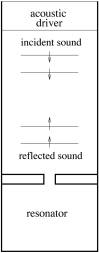
and then propose parallel computing methods accordingly. To illustrate the
idea, we will use the slit resonator in a two dimensional impedance tube as an
example. The configuration is shown by Fig.1. Details of the simulation are in Tam et.al.2005.
Serial Computing
Two
properties need to be taken into account when implementing a scheme with
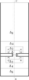
multi-size-mesh and multi-time-step. First, multi-size-mesh requires that the
physics domain be divided into subdomains (Fig.2). Grid size is uniform in each
subdomain. The smallest grid size, ![]() , is in subdomains around the slit mouth where viscous effect
is the strongest. Grid sizes are
increased in subdomains away from the slit mouth by a factor of 2, i.e.,
, is in subdomains around the slit mouth where viscous effect
is the strongest. Grid sizes are
increased in subdomains away from the slit mouth by a factor of 2, i.e.,![]() ,
, ![]() ,
, ![]() , etc. In the
simulation of the slit-resonator impedance tube in Tam et.al.2005, grid sizes up to
, etc. In the
simulation of the slit-resonator impedance tube in Tam et.al.2005, grid sizes up to ![]() are used. In
Fig.2 only grid sizes up to
are used. In
Fig.2 only grid sizes up to ![]() are shown for
clarity. For each subdomain, information outside of its boundaries is needed
before spatial derivatives can be computed. Therefore data exchanges are necessary
between adjacent subdomains.
are shown for
clarity. For each subdomain, information outside of its boundaries is needed
before spatial derivatives can be computed. Therefore data exchanges are necessary
between adjacent subdomains.
|
|
|
|
Fig.1, Slit
resonator in two-dimensional impedance tube. |
Fig.2, Subdomains
in the impedance tube. |
Second,
due to multiple time steps, the number of subdomains involved in computation is
different at different time level n. Subdomains
in which computations are performed at time ![]() are shown by
Fig.3(a). (
are shown by
Fig.3(a). (![]() in Fig.3.) At time level
in Fig.3.) At time level ![]() all the
subdomains are involved in the computation. At
all the
subdomains are involved in the computation. At ![]() computation is
done only in
computation is
done only in ![]() subdomains
(subdomains with grid size
subdomains
(subdomains with grid size ![]() ). At
). At ![]() ,
, ![]() and
and ![]() subdomains are
involved. The relation between physics time and CPU time is shown in Fig.4. It
is clear that the number of subdomains involved in computation, and thus CPU
time, is different at each time level n.
subdomains are
involved. The relation between physics time and CPU time is shown in Fig.4. It
is clear that the number of subdomains involved in computation, and thus CPU
time, is different at each time level n.
At
an interface between two subdomains with different grid sizes, flow variable
update at half time level is needed in the coarser subdomain. This updating
must be done before computing spatial derivatives in the finer subdomain.
Therefore the computation order at each time level is crucial. It should be from
coarser subdomains to finer subdomains for
Fig.3(a). For example, at ![]() ,
, ![]() subdomains must
be first computed, then
subdomains must
be first computed, then ![]() subdomains,
subdomains, ![]() subdomains, and
finally
subdomains, and
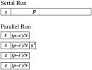
finally ![]() subdomains. In
each subdomain Fig.5 shows the computation sequence. Synchronization and data
exchange need to be done twice, which means two times of message passing (MPI)
or thread creating/terminating (OpenMP or Pthreads) are needed for parallel
computing.
subdomains. In
each subdomain Fig.5 shows the computation sequence. Synchronization and data
exchange need to be done twice, which means two times of message passing (MPI)
or thread creating/terminating (OpenMP or Pthreads) are needed for parallel
computing.
|
|
|
||||||||||||||||||||||||||||||||||||||||||||||||||||||||||||||||||||||||||||||||||||||||||||||||||||||||||||||||||||||
Fig.3, Subdomains
involved in simulation at different time levels.
![]()
Fig.4, Relation
between physics time and CPU time for Fig.3(a).
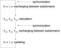
Fig.5,
Computation sequence in each subdomain.
Parallel
Partitioning
A single computation task can have multiple, concurrent
execution processes. One process handles part of subdomains (domain
decomposition), or part of the functions (function decomposition). Factors that
affect parallel efficiency are workload balance among processes, overhead of message
passing in MPI or thread creation/termination in multi-thread programming
(OpenMP and Pthreads).
Only domain decomposition model will be considered for
the impedance tube case. In a serial code, different number of subdomains are computed
at different time level (Fig.3(a), Fig.4). A partition, say, of ![]() and
and ![]() subdomains for process 1, and
subdomains for process 1, and ![]() and
and ![]() subdomains for
process 2, will make unbalanced workloads among processes even there are the
same amounts of grid points in both processes. For most of the time only
subdomains for
process 2, will make unbalanced workloads among processes even there are the
same amounts of grid points in both processes. For most of the time only ![]() and
and ![]() subdomains in
process 1 are involved in computation, and process 2 is idle mostly.
subdomains in
process 1 are involved in computation, and process 2 is idle mostly.
Partition on Subdomains of the Same Grid Size
One may separate the computation domain into 2 or 4 parts by line AB in the slit and the symmetric line CD, Fig.2. This partition distribute grid points of subdomains with the same grid size evenly among 2 or 4 processes. Data exchange between the two slit subdomains is only needed along AB. Structure of exchanging arrays along CD is consistent with the column-bases array data structure in FORTRAN. Partition between two processes along line AB is easy to program based on an existing serial code.
Partition across Subdomains with Different Grid
Sizes
Shown in Fig.3(a) is not the only computation order in
a serial code. Here we propose a different computation order in Fig.3(b). At
time level ![]()
![]() and
and ![]() subdomains are computed. At
subdomains are computed. At ![]() computation is
done in
computation is
done in ![]() and
and ![]() subdomains. At
subdomains. At ![]()
![]() and
and ![]() subdomains are
computed, et.al. The physics time ~ CPU
time relation is shown in Fig.6.
subdomains are
computed, et.al. The physics time ~ CPU
time relation is shown in Fig.6.
![]()
Fig.6,
Relation between physics time and CPU time for Fig.3(b).
At each time level the computation and data exchange
order is totally different from those in Fig.3(a). The computation must be
performed from finer subdomains to coarser subdomains. And in each subdomain it is not correct to obtain
information from finer subdomain. Instead one should transfer data from this
subdomain to its coarser neighbors. As an example, the correct orders for ![]() subdomain are: (1)
exchange
subdomain are: (1)
exchange ![]() between
between ![]() subdomains; (2) exchange
subdomains; (2) exchange
![]() between
between ![]() and
and ![]() subdomains; (3)exchange
subdomains; (3)exchange
![]() between
between ![]() subdomains if
necessary; (4) compute viscous terms
subdomains if
necessary; (4) compute viscous terms ![]() in
in ![]() subdomains and
near the interfaces in
subdomains and
near the interfaces in ![]() subdomains; (5) exchange
subdomains; (5) exchange
![]() between
between ![]() subdomains; (6) exchange
subdomains; (6) exchange
![]() between
between ![]() and
and ![]() subdomains; (7) exchange
subdomains; (7) exchange
![]() between
between ![]() subdomains is
necessary; (8) update
subdomains is
necessary; (8) update ![]() to the next time
level in
to the next time
level in ![]() subdomains.
subdomains.
The advantage of this new order is, the number of
subdomains involved at one time level is 2 most of the time. One may designate ![]() subdomains to
process 1 and all others to process 2. If message passing model is used, the
data exchange is needed along EFGH and PQRS in Fig.2, which may need more message passing CPU
time than the partition method on each domain. But as we will see later,
message passing time is very small compared to computation time. The advantage
of this partition is that it is easier to program based on a serial code.
subdomains to
process 1 and all others to process 2. If message passing model is used, the
data exchange is needed along EFGH and PQRS in Fig.2, which may need more message passing CPU
time than the partition method on each domain. But as we will see later,
message passing time is very small compared to computation time. The advantage
of this partition is that it is easier to program based on a serial code.
Combined Partition
The two partition methods, partition on subdomains with the same grid size and partition across subdomains with different grid sizes, can be combined to support 8 or more processes in this case.
Parallel
Computation Implementation
Parallel Programming Models
The computation was performed on the IBM RS/6000 SP3 supercomputer at Florida State University. IBM SP3 has a parallel architecture with hybrid shared and distributed memory. It is composed of 42 nodes, 4 CPUs on each node. Each node is a shared memory component, which can be viewed as a SMP (symmetric multiprocessor) machine. Processors on a SMP node can address that machine's memory as global. On the other hand, different nodes are separated machines between which communications are undertaken by network.
There are two different parallel programming models. MPI (message passing interface) treats all processors as single machines no matter if they are on the same node. Explicit data communication is needed among distributed memories on different machines. A MPI code is portable and scalable with large amount of processors. But it needs much effort on reprogramming serial codes, and data communication overhead needs to be taken into account.
Threads (multi-threaded programs) models are for shared memory machines. A thread is an independent control flow within the same address space as other independent control flows in a process. There are two threads models: OpenMP and Pthreads. In OpenMP a serial program is augmented with directives specifying which loops (sections) are to be parallelized. The compiler automatically creates threads for the loop (section) across SMP processors. It needs less labor on reprogramming and facilitates "incremented parallelism" for serial codes. On the other hand, in a Pthreads (POSIX) model, a process has to be threaded by hand using library functions. It needs explicit parallelism, but may have benefits when well done. No explicit data communication is needed for threads models. However they may be less portable (especially Pthreads). In cases of time dependent computational aeroacoustics (CAA), overhead of thread managing may be quite significant since at each time level threads have to be created and terminated dynamically.
IBM SP3 supports all the three parallel models (MPI, OpenMP, and Pthreads). When one task is partitioned over multiple nodes, MPI is the only choice. For processes within one node, OpenMP or Pthreads can also be used. For large application codes, experience indicates that MPI often works better than threads models. OpenMP is mostly useful on loop levels with iteration counts over 10000. If there are subroutine and function calls in the loop, variable scoping, which is the critical part of programming in threads models, becomes more difficult, and parallelization becomes less efficient or even worse than its serial version.
OpenMP or Pthreads is not suitable for the 2-D impedance tube case. Implementation shows that the code with OpenMP runs slower than the serial code. Therefore we will use MPI as our parallel model.
The domain partition strategy for the case is shown in Table 1.
Table
1, Domain Partition.
|
Number of Processes |
Separation Lines (Fig.2) |
|
2 |
AB |
|
4 |
AB&EFGH&PQRS |
|
8 |
AB&EFGH&PQRS&CD |
In the DRP scheme, there are roughly 388 operations to
solve N.S. equations at one time step. Each operation takes ![]() second of SP3
CPU. Therefore for a typical computation domain with
second of SP3
CPU. Therefore for a typical computation domain with ![]() grid points, the
computation time of one time step is:
grid points, the
computation time of one time step is:
![]() ~ 0.1 Second.
~ 0.1 Second.
Communication time is estimated by:
![]() .
.
Table 2 lists the latency and bandwidth of SP3. If the
interface of two grid subdomains has 100 grid points, the total grid points at
which data exchange is needed are ![]() . At each point there are 7 variables (
. At each point there are 7 variables (![]() ), 8 bytes each variable with double precision. Data needs to
be transferred twice (send and receive). Therefore the communication time on
different nodes is:
), 8 bytes each variable with double precision. Data needs to
be transferred twice (send and receive). Therefore the communication time on
different nodes is:
![]() ,
,
which is much small compared with the computation time.
Table
2, Latency and Bandwidth of IBM SP3
|
Protocol |
Location of 2 Processes |
Latency |
Bandwidth |
|
User Space |
On different nodes |
22 |
133 MB/Sec. |
|
On the same node |
37 |
72 MB/Sec. |
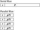
Suppose the fraction of running time for the part which
is not parallelized is s in a code. The
fraction of the remaining part, ![]() , is computed concurrently by N processes, Fig.7. Then speed up of the parallelization is defined as:
, is computed concurrently by N processes, Fig.7. Then speed up of the parallelization is defined as:
![]() .
.
|
|
|
|
Fig.7, Even workload among processes. |
Fig.8, Uneven workload among processes. |
Efficiency of the parallelization is defined as the
speed up divided by the number of processes N:
![]() .
.
Table 3 shows p
is extremely important for large number of processes. If p is small, the more processes are used, the more
processes are wasted.
Table
3, Speed Up and Efficiency of Parallelization
|
N |
|
|
|
|||
|
Speed Up |
Efficiency |
Speed Up |
Efficiency |
Speed Up |
Efficiency |
|
|
10 |
1.82 |
18.2% |
5.26 |
50.26% |
9.17 |
91.7% |
|
100 |
1.98 |
1.98% |
9.17 |
9.17% |
50.25 |
50.25% |
|
1000 |
1.99 |
0.199% |
9.91 |
0.991% |
90.99 |
9.099% |
|
10000 |
1.99 |
0.0199% |
9.91 |
0.0991% |
99.02 |
0.99% |
Uneven workload among processes has the same effect as
low p. Fig.8 shows an example of uneven
workload. Speed up of this parallelization is:
![]() .
.
Uneven workload ![]() lowers the
parallelization fraction dramatically and makes parallelization less effective.
lowers the
parallelization fraction dramatically and makes parallelization less effective.
For the impedance tube case, speed up of the 2
processes run (Table 1) is 1.9663, parallel efficiency 98.3%. For the 4
processes code, there are 10000 grid points for each of the two processes,
15738 grid points for each of the other two processes. Speed up is 3.1919,
parallel efficiency: 79.8%. The 8 processes code in Table 1 wasnπt implemented.
The techniques described in this section were also used
in simulations of three-dimensional slit resonators in impedance tube. (Tam et.al.2009)
References
Tam, C.K.W., and Kurbatskii,
K.A., Multi-size-mesh Multi-time-step Dispersion-Relation-Preserving Scheme for
Muliple-Scales Aeroacoustics Problems, International Journal of
Computational Fluid Dynamics, Vol.17, 2003,
pp. 119-132.
Tam, C.K.W., Ju, H., Jones,
M.G., Watson, W.R., and Parrott, T.L., A Computational and Experimental Study
of Slit Resonators, Journal of Sound and Vibration, Vol. 284, 2005, pp. 947-984.
Tam, C.K.W., Ju, H., Jones,
M.G., Watson, W.R., and Parrott, T.L., A Computational and Experimental Study
of Resonators in Three Dimensions, AIAA-2009-3171.
RS/6000 SP: Practical MPI
Programming, International Technical Support Organization, www.redbooks,ibm.com.
Scientific Applications in
RS/6000 SP Environments, International Technical Support Organization,
www.redbooks.ibm.com.