Waves in Uniform Flow on Half Plane
Hongbin Ju
Department of Mathematics
Florida State University, Tallahassee, FL.32306
www.aeroacoustics.info
Please send comments to: hju@math.fsu.edu
The
normal mode method is employed to identify normal modes of linear Euler
equations in uniform mean flow. The physical domain is a two-dimensional half
open space. Three normal modes: acoustic wave, vorticity wave, and entropy
wave, are explored and discussed.
Mean Flow Parallel to the Interface
Linear Euler
Equations and the Normal Mode Method
The
Euler equations for an ideal adiabatic gas are:
![]() ,
(1)
,
(1)
![]() ,
(2)
,
(2)
![]() ,
(3)
,
(3)
![]() .
(4)
.
(4)
Consider
the uniform mean velocity ![]() in x direction. Quantities with prime
represent perturbation, and those with subscript 0 represent ambient values:
in x direction. Quantities with prime
represent perturbation, and those with subscript 0 represent ambient values: ![]() ,
, ![]() ,
, ![]() , etc. The perturbation is small compared with the ambient
quantities, so that the linearized equations apply:
, etc. The perturbation is small compared with the ambient
quantities, so that the linearized equations apply:
![]() ,
(5)
,
(5)
![]() ,
(6)
,
(6)
![]() ,
(7)
,
(7)
![]() . (8)
. (8)
where ![]() .
.
Consider
the mean flow parallel to the interface ![]() . The half space is above x-axis. The physical domain is:
. The half space is above x-axis. The physical domain is:
![]() ,
, ![]() .
.
We
will use the normal mode method to solve the problem. The normal mode method
can identify all the normal modes of a system. The normal modes are building
blocks for the solutions of the Euler equations with an initial field.
Instabilities and its characteristics can also be identified with this method.
The
mean flow is homogeneous and the physical domain extends infinitely in x direction. One can use exponential
functions as the trial solutions on x and t
and assume the next form of
solution:
 .
(9)
.
(9)
Substituting
(9) into linear Euler equations (5)~(8), one obtains:
![]() ,
(10)
,
(10)
![]() ,
(11)
,
(11)
![]() ,
(12)
,
(12)
![]() ,
(13)
,
(13)
 .
(14)
.
(14)
Acoustic Wave
Now
one needs to solve ![]() ,
,![]() , and
, and ![]() from (10)~(14).
First assume
from (10)~(14).
First assume ![]() , then one has:
, then one has:
![]() ,
(15)
,
(15)
![]() ,
(16)
,
(16)
![]() ,
(17)
,
(17)
![]() .
(18)
.
(18)
where
![]() ,
, ![]() .
(19)
.
(19)
We
will choose appropriate branch cuts of ![]() in
in ![]() -plane to ensure that
-plane to ensure that ![]() always has
nonnegative imaginary part:
always has
nonnegative imaginary part:
![]() .
.
Then
the general solution to Eq.(15) is:
![]() .
(20)
.
(20)
A and B are to be determined by boundary
conditions at ![]() and
and ![]() .
.
From
Eqs.(16) and (17), vorticity on the half space is zero:
![]() ,
, ![]() .
(21)
.
(21)
There
is no entropy either in this solution, Eq.(18). Therefore this set of solutions
represents only acoustics waves. With subscript a, the acoustic solutions can be written
as:
![]() ,
(22)
,
(22)
![]() ,
(23)
,
(23)
![]() ,
(24)
,
(24)
![]() ,
, ![]() .
(25)
.
(25)
In
this set of equations, A
and B are determined
by boundary conditions at ![]() and
and ![]() .
. ![]() is computed from
Eq.(19). Eq.(19) is the
relation between frequency
is computed from
Eq.(19). Eq.(19) is the
relation between frequency ![]() and wave numbers
and wave numbers
![]() and
and ![]() . It is the dispersion relation for sound waves. In general,
. It is the dispersion relation for sound waves. In general, ![]() and
and ![]() can be any
complex numbers. If they are Fourier Transform variables, which means
Eqs.(10)~(14) are Fourier Transforms of Eqs.(5)~(8), then
can be any
complex numbers. If they are Fourier Transform variables, which means
Eqs.(10)~(14) are Fourier Transforms of Eqs.(5)~(8), then ![]() and
and ![]() are real
numbers. To illustrate how to compute
are real
numbers. To illustrate how to compute ![]() , we will assume
, we will assume ![]() and
and ![]() are real. From
(19), depending on
are real. From
(19), depending on ![]() , there are three situations for choosing the branch cuts in
, there are three situations for choosing the branch cuts in ![]() -plane to determine
-plane to determine ![]() .
.
If
![]() ,
, ![]() is real and
positive, choose the branch cuts as in Fig.1:
is real and
positive, choose the branch cuts as in Fig.1:
![]() ,
, ![]() . (26)
. (26)
With
these branch cuts, the imaginary part of ![]() is non-negative.
is non-negative.
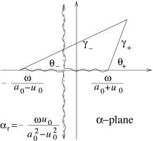
Fig.1, Branch cuts in ![]() -plane when
-plane when ![]() ,
, ![]() is real and
positive.
is real and
positive.
When
![]() is real,
is real,
 .
(27)
.
(27)
For
incompressible flow, ![]() ,
,
![]() (28)
(28)
From
Eq.(22), the time domain sound pressure is:
![]() .
(29)
.
(29)
When
![]() is real and
is real and ![]() ,
, ![]() is real and
Eq.(29) represents two propagating plane waves. Plane wave
is real and
Eq.(29) represents two propagating plane waves. Plane wave ![]() propagates to
the far field
propagates to
the far field ![]() ; plane wave
; plane wave ![]() propagates
towards the boundary at
propagates
towards the boundary at ![]() . The propagation angle of plane wave
. The propagation angle of plane wave ![]() as
as ![]() changes from 0
to
changes from 0
to ![]() is shown in Fig.2.
The wave propagates normal to the interface to the far field when
is shown in Fig.2.
The wave propagates normal to the interface to the far field when ![]() , Fig.3(a). As
, Fig.3(a). As ![]() increases, the
wave slants toward the flow direction, Fig.3(b). Eventually the wave propagates
along the interface when
increases, the
wave slants toward the flow direction, Fig.3(b). Eventually the wave propagates
along the interface when ![]() , Fig.3(c). The wave amplitude is constant along the phase
perpendicular to the propagation direction. Phase speed of the wave is
, Fig.3(c). The wave amplitude is constant along the phase
perpendicular to the propagation direction. Phase speed of the wave is ![]() , shown in Fig.4. It increases from
, shown in Fig.4. It increases from ![]() to maximum
to maximum ![]() as
as ![]() changes from 0
to
changes from 0
to ![]() . In this
. In this ![]() range, the phase
speed of the wave in x
direction ,
range, the phase
speed of the wave in x
direction , ![]() , is supersonic.
, is supersonic.
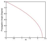
Fig.2, Plane wave propagation angle vs. ![]() . (
. (![]() ,
, ![]() )
)
![]()
![]()
![]()
(a) ![]() (b)
(b)
![]() (c)
(c) ![]()
Fig.3, Plane waves for ![]() .
.
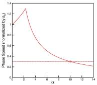
Fig.4, Phase speed vs. ![]() . (
. (![]() ,
, ![]() )
)
When
![]() and
and ![]() , or
, or ![]() ,
, ![]() is purely
imaginary. Fig.5 shows the variation of
is purely
imaginary. Fig.5 shows the variation of ![]() as
as ![]() . The wave pattern is shown in Fig.6. The wave only
propagates in x
direction and the amplitude decays in y direction. The effect of disturbances is local to the
interface. In this
. The wave pattern is shown in Fig.6. The wave only
propagates in x
direction and the amplitude decays in y direction. The effect of disturbances is local to the
interface. In this ![]() range, the wave
doesn't propagate to the far field. Phase speed of the wave is subsonic:
range, the wave
doesn't propagate to the far field. Phase speed of the wave is subsonic: ![]() , which is not related to sound speed
, which is not related to sound speed ![]() . Fig.4 shows that the phase speed decreases as
. Fig.4 shows that the phase speed decreases as ![]() increases from
increases from![]() . This is the only wave pattern for incompressible flow.
(Check out sound wave reflection/transmission at density interface, the
vortex/shock wave interaction, where this kind of wave is excited.)
. This is the only wave pattern for incompressible flow.
(Check out sound wave reflection/transmission at density interface, the
vortex/shock wave interaction, where this kind of wave is excited.)
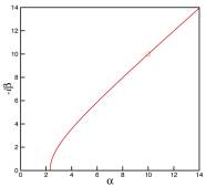
Fig.5, Imaginary ![]() for
for ![]() and
and ![]() .
.
![]()
Fig.6, waves for ![]() and
and ![]() .
.
In
the above analysis, ![]() is assumed. When
is assumed. When
![]() , the phase speed is equal to the mean flow velocity. This
point is indicated by a circle In Figs.(4)&(5). Mathematically this is a
singular point for acoustic equations (15)~(17). As
, the phase speed is equal to the mean flow velocity. This
point is indicated by a circle In Figs.(4)&(5). Mathematically this is a
singular point for acoustic equations (15)~(17). As ![]() , acoustic velocities approach infinity. In physics this
corresponds to the resonance phenomena. In this case the exponential functions
we used as the trial solutions are not suitable. We have to use other trial
functions, or appeal to Laplace Transform method. However even the mathematical
solution is possible, there is no physically acceptable acoustic solution. The
physical model (invisid and linear) breaks down. The sound wave can not be
damped by viscosity; it grows infinitively due to linearity. One way to obtain
a physically acceptable acoustic solution is to use a better model including
viscosity and nonlinearity, such as the full N.S. equations. Another way is to
appeal to analytical continuation.
, acoustic velocities approach infinity. In physics this
corresponds to the resonance phenomena. In this case the exponential functions
we used as the trial solutions are not suitable. We have to use other trial
functions, or appeal to Laplace Transform method. However even the mathematical
solution is possible, there is no physically acceptable acoustic solution. The
physical model (invisid and linear) breaks down. The sound wave can not be
damped by viscosity; it grows infinitively due to linearity. One way to obtain
a physically acceptable acoustic solution is to use a better model including
viscosity and nonlinearity, such as the full N.S. equations. Another way is to
appeal to analytical continuation. ![]() can be treated
as a complex number with positive
imaginary part, and the integration path in the Inverse Fourier Transform
should be detoured accordingly to avoid the singular point. This is equivalent
to introduce artificial damping into the system, or apply Laplace Transform on t. In Laplace transform method
can be treated
as a complex number with positive
imaginary part, and the integration path in the Inverse Fourier Transform
should be detoured accordingly to avoid the singular point. This is equivalent
to introduce artificial damping into the system, or apply Laplace Transform on t. In Laplace transform method ![]() is the
Laplace transform variable, whose integral contour is above all singularities.
The inverse Laplace transform has no singularity problem along this integral
contour.
is the
Laplace transform variable, whose integral contour is above all singularities.
The inverse Laplace transform has no singularity problem along this integral
contour.
For
a complex ![]() , the wave is a decayed plane wave propagating in an oblige
direction.
, the wave is a decayed plane wave propagating in an oblige
direction.
If
![]() , choose the branch cut is as in Fig.7:
, choose the branch cut is as in Fig.7:
![]() .
(30)
.
(30)
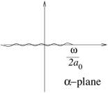
Fig.7, Branch cut in ![]() -plane when
-plane when ![]() .
.
If
![]() , choose the branch cuts as in the Fig.8:
, choose the branch cuts as in the Fig.8:
![]() ,
, ![]() .
(31)
.
(31)
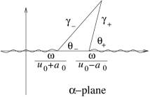
Fig.8, Branch cuts in ![]() -plane when
-plane when ![]() .
.
An
important property of acoustic wave can be derived from Eqs.(10), (11) and
(12):
![]() .
.
Since
![]() and
and ![]() are real,
are real,
![]() .
(32)
.
(32)
![]() is the time
averaged acoustic kinetic energy, and
is the time
averaged acoustic kinetic energy, and ![]() the time
averaged acoustic potential energy. Eq.(32) means that the time averages of acoustic kinetic energy and
potential energy are equal.
the time
averaged acoustic potential energy. Eq.(32) means that the time averages of acoustic kinetic energy and
potential energy are equal.
Vorticity
Wave
Now
let's assume:
![]() .
(33)
.
(33)
If
![]() or
or ![]() , then
, then ![]() , the solution will be time-invariant, which is of no
interest in the discussion. Therefore we can further assume
, the solution will be time-invariant, which is of no
interest in the discussion. Therefore we can further assume ![]() and
and ![]() . The next equations can be derived from (10)~(14):
. The next equations can be derived from (10)~(14):
![]() ,
(34)
,
(34)
![]() ,
(35)
,
(35)
![]() .
(36)
.
(36)
From
Eq.(34), there is no pressure fluctuations in this solution. From (35) and
(36), velocities ![]() and
and ![]() , and thermodynamic variable
, and thermodynamic variable ![]() can be
determined separately.
can be
determined separately.
First
we discuss the velocity solution. One has this set of solutions:
![]() ,
(37)
,
(37)
![]() ,
(38)
,
(38)
![]() ,
(39)
,
(39)
![]() .
(40)
.
(40)
![]() is function of y. It can be set at any line
is function of y. It can be set at any line ![]() . Usually it is determined at upstream boundary.
. Usually it is determined at upstream boundary.
The
vorticity is
![]() ,
(41)
,
(41)
and the dilation
![]() ,
, ![]() =0.
(42)
=0.
(42)
This
solution is dilation free. It represents a vorticity wave, which is denoted by
subscript v. Eq.(33)
is the dispersion relation for vorticity waves.
One
can study one Fourier component of the vorticity wave:
![]() ,
(43)
,
(43)
![]() .
(44)
.
(44)
Since
![]() , the velocity direction is perpendicular to the wave
propagation direction. Therefore a vorticity wave is a transverse wave.
, the velocity direction is perpendicular to the wave
propagation direction. Therefore a vorticity wave is a transverse wave.
Entropy
Wave
The
other set of solution to Eqs.(34)~(36), is:
![]() ,
(45)
,
(45)
![]() ,
(46)
,
(46)
![]() ,
(47)
,
(47)
![]() (48)
(48)
Similar to ![]() ,
, ![]() can be determined at the upstream
boundary. In this set of solutions only heat is involved. It is the entropy wave. An entropy wave
only consists entropy fluctuation, or density fluctuation
can be determined at the upstream
boundary. In this set of solutions only heat is involved. It is the entropy wave. An entropy wave
only consists entropy fluctuation, or density fluctuation ![]() . Eq.(33) is also the dispersion relation
for entropy waves.
. Eq.(33) is also the dispersion relation
for entropy waves.
Solutions
in Time Domain
In
the uniform mean flow, the three normal modes: acoustic, vorticity and entropy
waves, have been identified. Once four boundary conditions are set: ![]() and
and ![]() at the upstream boundary,
at the upstream boundary, ![]() and
and ![]() at
at ![]() and
and ![]() , the three waves for each pair of
, the three waves for each pair of ![]() are uniquely
determined from Eqs.(22)~(25), Eqs. (37)~(40), and Eqs. (45)~(48). Then the
total solution for this
are uniquely
determined from Eqs.(22)~(25), Eqs. (37)~(40), and Eqs. (45)~(48). Then the
total solution for this ![]() and
and ![]() is:
is:
![]() ,
, ![]() ,
, ![]() . (49)
. (49)
In
all the boundary conditions if there is no complex ![]() with positive
imaginary part for any real
with positive
imaginary part for any real ![]() , there are no instabilities. Then the normal mode analysis
is equivalent to the Fourier Transform method, and the time domain solutions
can be obtained by the Inverse Fourier Transform. For example, the time domain
pressure is:
, there are no instabilities. Then the normal mode analysis
is equivalent to the Fourier Transform method, and the time domain solutions
can be obtained by the Inverse Fourier Transform. For example, the time domain
pressure is:
![]() .
.
Mean Flow Perpendicular to the
Interface
In
this section we will consider the mean flow that is perpendicular to the
interface. Mean flow ![]() is in
is in ![]() direction. The
half open space is:
direction. The
half open space is:
![]() ,
, ![]() .
.
The
physical domain extends infinitely in y direction. The normal mode method will be applied on y and t. Consider the next form of solutions:
 .
(50)
.
(50)
![]() and
and ![]() are real numbers. Substituting (50) into
linear Euler equations (5)~(8), one has:
are real numbers. Substituting (50) into
linear Euler equations (5)~(8), one has:
![]() ,
(51)
,
(51)
![]() ,
(52)
,
(52)
![]() ,
(53)
,
(53)
![]() ,
(54)
,
(54)
![]() .
(55)
.
(55)
Acoustic Wave
To
eliminate ![]() and
and ![]() from (51), one
can apply
from (51), one
can apply ![]() on (51) and plug
(52) and (53) into the equation to obtain:
on (51) and plug
(52) and (53) into the equation to obtain:
![]() .
(56)
.
(56)
This is a homogeneous linear
second order ordinary differential equation
when ![]() . There is a trivial solution
. There is a trivial solution ![]() . But first we will discuss the nontrivial solution.
. But first we will discuss the nontrivial solution.
If ![]() , the nontrivial solution of (56) is:
, the nontrivial solution of (56) is:
![]() ,
(57)
,
(57)
![]() .
(58)
.
(58)
![]() and
and ![]() are to be
determined by boundary conditions at
are to be
determined by boundary conditions at ![]() and
and ![]() .
.
The
branch cuts of ![]() in
in ![]() -plane are shown in the Fig.9:
-plane are shown in the Fig.9:
![]() ,
, ![]() .
(59)
.
(59)
![]() always has
positive imaginary part, and
always has
positive imaginary part, and ![]() always has
negative imaginary part.
always has
negative imaginary part.
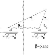
Fig.9, Branch cuts in ![]() -plane when
-plane when ![]() .
.
Since
![]() is real:
is real:
 (60)
(60)
When
![]() ,
, ![]() are real and the
waves are pure propagating plane waves. When
are real and the
waves are pure propagating plane waves. When ![]() , the wave only
propagates in y
direction with phase speed
, the wave only
propagates in y
direction with phase speed ![]() , and the amplitude decays in x direction; disturbances are only local
near the interface. For
, and the amplitude decays in x direction; disturbances are only local
near the interface. For ![]() with imaginary
part, the wave is decayed plane waves propagating in an oblige direction.
with imaginary
part, the wave is decayed plane waves propagating in an oblige direction.
Acoustic
wave is an isentropic process. Therefore the set of acoustic solutions is:
![]() ,
(61)
,
(61)
![]() ,
(62)
,
(62)
![]() ,
(63)
,
(63)
![]() ,
, ![]() .
(64)
.
(64)
There
is no entropy in the solution from Eq.(64). One can show that the vorticity in
the physical domain is zero:
![]() ,
, ![]() .
(65)
.
(65)
So
this set of solutions only represent acoustics waves (denoted by subscript a), excluding any vortical and heat
motions in the physical domain.
If
![]() ,
,
![]() .
(66)
.
(66)
The
branch cut of ![]() in
in ![]() -plane is shown in Fig.10, so that
-plane is shown in Fig.10, so that ![]() always has
positive imaginary part, and
always has
positive imaginary part, and ![]() always has
negative imaginary part.
always has
negative imaginary part.
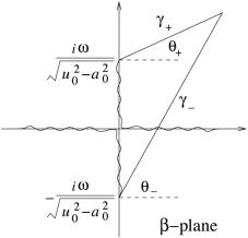
Fig.10, Branch cuts in ![]() -plane when
-plane when ![]() .
.
If
![]() , Eq.(56) degenerates to a first order PDE with the
nontrivial solution:
, Eq.(56) degenerates to a first order PDE with the
nontrivial solution:
![]() ,
, ![]() .
(67)
.
(67)
Vorticity
wave
Now we return to the trivial solution of (56):
![]() .
(68)
.
(68)
Plugging (68) into (51)~(53), we have:
![]() ,
(69)
,
(69)
![]() ,
(70)
,
(70)
![]() .
(71)
.
(71)
Eq.(69)
means it is dilation free. The solutions of the vortical wave are:
![]() ,
(72)
,
(72)
![]() ,
(73)
,
(73)
![]() ,
(74)
,
(74)
![]() .
(75)
.
(75)
![]() should be determined by upstream
boundary condition.
should be determined by upstream
boundary condition.
Entropy
Wave
The
other set of solutions is:
![]() ,
(76)
,
(76)
![]() ,
(77)
,
(77)
![]() ,
(78)
,
(78)
![]() ,
, ![]() .
(79)
.
(79)
Once the four boundary conditions: three at upstream boundary and one at downstream boundary, are set, unique solutions for acoustic, vorticity, and entropy waves will be determined.