Acoustic Wave
Hongbin Ju
www.aeroacoustics.info
hju@math.fsu.edu
The discussion of different modes and their interactions provides important information on sound sources. Once the sound sources are determined, the next task is to obtain the sound fields by solving the acoustic wave equations. In this chapter we study how to solve the sound field in an open space. (Sound in ducts is to be discussed in a separate chapter.) The sound field from a pulsating sphere in a three-dimensional (3-D) space is first investigated. The concepts of monopole, dipole and quadrupole are introduced. Based on the monopole sound solution, one of the most important techniques to solve acoustic equations is introduced: the 3-D Green’s function and the formal integral solutions. Using the integral solutions, the sound field from moving sources, especially rotating sources, is studied. The two-dimensional (2-D) Green’s function is also briefly discussed.
Acoustic Wave Equations
For the acoustic mode in a uniform ideal flow:
![]() ,
(2)
,
(2)
![]() .
(4)
.
(4)
These
are the irrotational, isentropic, linear Euler equations. Variables with
subscript ‘0’ are mean flow quantities, and ![]() . All
other variables are perturbation variables.
. All
other variables are perturbation variables.
Velocity Potential and Acoustic Wave Equations
The
most important consequence of Eq.(4) (![]() ) is
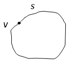
the introduction of the velocity potential. Shown in Fig. 1 is a control volume
V bounded by inner surface
) is
the introduction of the velocity potential. Shown in Fig. 1 is a control volume
V bounded by inner surface ![]() and outer surface
and outer surface ![]() . C is a closed contour in V.
C is reducible if it can shrink to a point without having to cross any
boundaries. Its shrinking path forms a surface
. C is a closed contour in V.
C is reducible if it can shrink to a point without having to cross any
boundaries. Its shrinking path forms a surface ![]() . If
in V any contour is reducible, the region is singly-connected.
Otherwise, it is multiply-connected. If the volume in Fig.1 is three-dimensional
and the dimensions of the inner body are finite, then V if singly-connected.
On the other hand, if the volume is two-dimensional, the inner body extends to
infinity in the third direction. Any contour enclosing the body is not
reducible; therefore V is multiply-connected. This argument shows the
difference of the mathematical treatment when dealing with two-dimensional and
three-dimensional problems.
. If
in V any contour is reducible, the region is singly-connected.
Otherwise, it is multiply-connected. If the volume in Fig.1 is three-dimensional
and the dimensions of the inner body are finite, then V if singly-connected.
On the other hand, if the volume is two-dimensional, the inner body extends to
infinity in the third direction. Any contour enclosing the body is not
reducible; therefore V is multiply-connected. This argument shows the
difference of the mathematical treatment when dealing with two-dimensional and
three-dimensional problems.
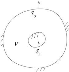
Fig. 1, Control
volume V bounded by inner surface ![]() and
outer surface
and
outer surface ![]() .
.
Suppose
in a singly-connected region there are two points O and P, and
two paths ![]() and
and ![]() joining
the two points.
joining
the two points. ![]() and
and ![]() forms
a closed contour
forms
a closed contour ![]() and there exists a surface
and there exists a surface ![]() with contour C as the boundary.
By applying the Stokes’ theorem, we know that circulation
with contour C as the boundary.
By applying the Stokes’ theorem, we know that circulation ![]() around the contour is zero since
around the contour is zero since ![]() . Therefore,
. Therefore,
![]() .
(5)
.
(5)
That
means the line integration is only a function of the positions of O and P.
It does not depend on the paths. Therefore, we can define a function of position
![]() :
:
![]() .
(6)
.
(6)
When
P approaches O, ![]() , we have:
, we have:
![]() .
.
As ![]() ,
, ![]() , then,
, then,
![]() .
(7)
.
(7)
![]() is the velocity potential function. Acoustic
velocity is the gradient of the velocity potential.
is the velocity potential function. Acoustic
velocity is the gradient of the velocity potential.
In a
multiply-connected region, contour ![]() may not be reducible.
Under this circumstance, the Stokes’ Theorem doesn’t apply and circulation
may not be reducible.
Under this circumstance, the Stokes’ Theorem doesn’t apply and circulation ![]() around C may not be zero even for
around C may not be zero even for
![]() . Then,
. Then,
![]() .
.
The
line integration depends on the path going from O to P. Velocity
potential ![]() defined by Eq.(6) has multiple values at
a point depending on how many rounds the path goes.
defined by Eq.(6) has multiple values at
a point depending on how many rounds the path goes. ![]() is no
longer a function of position since it may have multiple values at the same
position. In this case, an artificial barrier, such as
is no
longer a function of position since it may have multiple values at the same
position. In this case, an artificial barrier, such as ![]() in
Fig. 2, must be inserted to make the region singly-connected.
in
Fig. 2, must be inserted to make the region singly-connected.
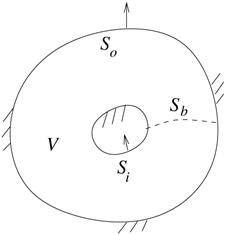
Fig.2, Artificial barrier in a multiply-connected control volume.
The
benefit of introducing the velocity potential is twofold: the number of
variables is reduced, and the irrotational requirement is automatically
satisfied since ![]() . One disadvantage is that
mathematically the velocity potential requires higher order smoothness than the
velocity itself.
. One disadvantage is that
mathematically the velocity potential requires higher order smoothness than the
velocity itself.
It
is the gradient of velocity potential, ![]() , not
the potential itself, that has physical meaning. Since
, not
the potential itself, that has physical meaning. Since ![]() is
defined by the spatial integral [Eq.(6)], any function of time
is
defined by the spatial integral [Eq.(6)], any function of time ![]() added to
added to ![]() does not
affect the equation and analysis.
does not
affect the equation and analysis.
With the newly introduced velocity potential, Eqs.(1) and (2) can be written as:
![]() ,
(8)
,
(8)
![]() ,
(9)
,
(9)
Assume the acoustic medium is uniform. Then the derivatives on the left side of Momentum equation Eq.(9) can be interchanged. Eq.(9) can be reduced to:
![]() ,
,
i.e.,
![]() ,
(10)
,
(10)
where
![]() is any function of time. According to
Eq.(7), any function of time added to
is any function of time. According to
Eq.(7), any function of time added to ![]() doesn’t
affect the acoustic velocity. Therefore, Eq.(10) can be written simply as:
doesn’t
affect the acoustic velocity. Therefore, Eq.(10) can be written simply as:
![]() .
(11)
.
(11)
Substituting it into continuity equation (9), we have:
![]() ,
(12)
,
(12)
![]() .
(13)
.
(13)
where
![]() .
.
These
are the acoustic equations in a uniform mean flow. It is also satisfied by any
other acoustic variables such as ![]() [51].
The nontrivial solution of (12) or (13) is the acoustic wave. The trivial
solution,
[51].
The nontrivial solution of (12) or (13) is the acoustic wave. The trivial
solution, ![]() or
or ![]() ,
corresponds to vorticity waves or entropy wave[52]s.
,
corresponds to vorticity waves or entropy wave[52]s.
There
are no sources in linear Euler equations (1) ~ (3). The corresponding acoustic
equation (13) or (12) is a homogeneous partial differential equation. It
describes the propagation of sound waves in a uniform flow. At any point in the
medium, ![]() must be zero. Otherwise, there are sound
sources at this point. These sources are from external action such as flow
injection, or from scattering of other modes due to nonuniformity in the flow,
or from nonlinear interactions between different modes.
must be zero. Otherwise, there are sound
sources at this point. These sources are from external action such as flow
injection, or from scattering of other modes due to nonuniformity in the flow,
or from nonlinear interactions between different modes.
Solution Uniqueness and Boundary Conditions
In a
singly connected region, Eq.(13) has a unique solution if the normal velocity
on all the boundary surfaces (![]() and
and ![]() in Fig.1) enclosing the area of interest
is prescribed (cht7.doc). The uniqueness of the solution can be proved by the
energy integral method (Pierce1989 p.171, Bachelor Chapter 2.7&2.8). If the
outside surface
in Fig.1) enclosing the area of interest
is prescribed (cht7.doc). The uniqueness of the solution can be proved by the
energy integral method (Pierce1989 p.171, Bachelor Chapter 2.7&2.8). If the
outside surface ![]() is at infinity, the sound
field vanishes according to the causality requirement. Causality means there is
no sound before it reaches the observer.
is at infinity, the sound
field vanishes according to the causality requirement. Causality means there is
no sound before it reaches the observer.
If
the region is multiply connected, we first make it singly connected by
inserting barrier(s) as in Fig. 2. Then the solution is unique when the normal
velocity distribution is prescribed on all surfaces: ![]() ,
,
![]() and barrier
and barrier ![]() . Prescribing
normal velocity on
. Prescribing
normal velocity on ![]() is equivalent to set the flux
across the artificial barrier, or circulation around the inner body. What is the
correct circulation for a particular problem? The model we began with [Eqs.(1)~(4)]
assumes inviscid medium. If the inner body surface is smooth, zero circulation
is often assumed (Morse&Ingard1968, p.400). If there is a sharp edge on the
inner surface, velocity at the sharp edge goes to infinity if the medium is
inviscid. In this case viscosity can not be neglected near the sharp edge. Vortexes
evolve and shed at the sharp edge due to the effect of viscosity; the
circulation is induced around the inner boundary. Therefore enforcing the Kutta
condition at the sharp edge is the way to set the exact circulation due to the viscous
effect. But this condition can only be applied once at one sharp edge, such as
the trailing edge of an airfoil. Discontinuity/infinity is allowed at other
sharp edges such as the leading edge of the airfoil.
is equivalent to set the flux
across the artificial barrier, or circulation around the inner body. What is the
correct circulation for a particular problem? The model we began with [Eqs.(1)~(4)]
assumes inviscid medium. If the inner body surface is smooth, zero circulation
is often assumed (Morse&Ingard1968, p.400). If there is a sharp edge on the
inner surface, velocity at the sharp edge goes to infinity if the medium is
inviscid. In this case viscosity can not be neglected near the sharp edge. Vortexes
evolve and shed at the sharp edge due to the effect of viscosity; the
circulation is induced around the inner boundary. Therefore enforcing the Kutta
condition at the sharp edge is the way to set the exact circulation due to the viscous
effect. But this condition can only be applied once at one sharp edge, such as
the trailing edge of an airfoil. Discontinuity/infinity is allowed at other
sharp edges such as the leading edge of the airfoil.
Prescribing normal velocity is only a sufficient, not necessary, boundary condition. A unique solution can also be rendered if velocity potential, or pressure, is set on the surfaces. Actually, a linear combination of the normal velocity and pressure can be given at the boundary surfaces. This is the impedance boundary condition, which will be discussed in another chapter.
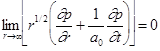
In an
open space, the outer surface ![]() is at infinity. In
numerical analyses, it is impossible to set the computation domain to infinity.
Usually the boundary is placed far away from the source region and approximate
equations are used to ensure causality, such as the Sommerfeld Radiation
Boundary equations:
is at infinity. In
numerical analyses, it is impossible to set the computation domain to infinity.
Usually the boundary is placed far away from the source region and approximate
equations are used to ensure causality, such as the Sommerfeld Radiation
Boundary equations:
 for
a 2-D stationary medium, (14)
for
a 2-D stationary medium, (14)
 for
a 3-D stationary medium, (15)
for
a 3-D stationary medium, (15)
or the 2D radiation boundary condition considering a mean flow by Tam:
![]() ,
,
![]() . (16)
. (16)
It is noted that Eq.(16) is different from (14) when M=0. These boundary conditions formally make an open region finite.
Sound Generated by Vibrating Spheres
Sound Generated by Radially Vibrating Sphere
in Stationary Medium (Mass Fluctuation)
Here we will discuss the sound field in a stationary medium generated by an external source: a vibrating sphere. Consider a sphere with radius R. The sphere surface vibrates radially with uniform amplitude and phase. When the vibration amplitude is small, the boundary condition can be represented by a uniform velocity at the nominal surface:
![]() at
at
![]() . (17)
. (17)
According to the uniqueness of solution discussed in the previous section, the sound field is uniquely determined with the boundary condition in (17).
In the spherical coordinate system, the gradient and the Laplacian are respectively:
![]() ,
,
![]() .
.
The boundary velocity in (17) and the sound field are spherically symmetric. Therefore wave equation (12) and (11) can be simplified:
![]() ,
(18)
,
(18)
![]() .
(19)
.
(19)
The general solution (the d’Alembert’s solution) of (18) is:
![]() .
(20)
.
(20)
F and E are two arbitrary functions representing respectively the out-going and in-coming spherical waves. The requirement of causality excludes function E. Therefore the solution is:
![]() ,
(21)
,
(21)
![]() ,
,
![]() ,
, ![]() ,
(22)
,
(22)
![]() ,
(23)
,
(23)
where
![]() .
.
The sound source is the mechanical vibration of the sphere. The volume of the sphere changes as its surface vibrates. It is equivalent to the injection of fluid into the medium. The rate of the injected volume is
![]() .
(24)
.
(24)
Substituting (22) into boundary condition (17), we have
![]() .
(25)
.
(25)
The first order linear ordinary
differential equation (ODE) (25) can be solved using the method of
separation of variables and the method of variation of parameter
(c.f. Appendix). Suppose there is no vibration at ![]() , then
the solution is:
, then
the solution is:
![]() .
(26)
.
(26)
Therefore the transient velocity potential is:
![]() ,
,
![]() ; (27)
; (27)
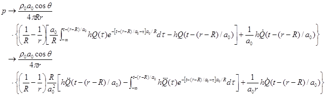
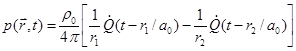
and the sound pressure:
![]() ,
,
![]() . (28)
. (28)
![]() is the retarded time at the surface
point closest to the observer. (27) and (28) give the sound field generated by
a vibrating sphere. They apply anywhere as long as
is the retarded time at the surface
point closest to the observer. (27) and (28) give the sound field generated by
a vibrating sphere. They apply anywhere as long as ![]() .
There is no physical and mathematical meaning for
.
There is no physical and mathematical meaning for ![]() . The
net force of the sphere acting on the fluid is zero since the pressure is
spherically symmetric.
. The
net force of the sphere acting on the fluid is zero since the pressure is
spherically symmetric.
Monopole
The
source is compact when its dimension is small compared with sound wavelength ![]() , i.e.,
, i.e., ![]() .
It is useful to investigate the sound field for a compact source. We assume the
amplitude of volume injection rate
.
It is useful to investigate the sound field for a compact source. We assume the
amplitude of volume injection rate ![]() is constant when the sphere shrinks into a point
is constant when the sphere shrinks into a point![]() .
Performing integration by parts we have,
.
Performing integration by parts we have,
 .
.
Note
![]() ,
,
then,
as ![]() ,
,
This approximation is very important and will be used repeatedly hereafter.
Apply
(29) in (27) and (28), then ![]() ,
,
![]() ,
,
![]() , (31)
, (31)
where
![]() . Eqs.(30)~(32) describe the sound field
from a compact source, i.e., source pulsating at low frequencies.
Actually they apply for any frequency, since the source region is reduced to a conceptual
point. This source is called monopole. The directivity of the sound field from
a monopole is omnidirectional.
. Eqs.(30)~(32) describe the sound field
from a compact source, i.e., source pulsating at low frequencies.
Actually they apply for any frequency, since the source region is reduced to a conceptual
point. This source is called monopole. The directivity of the sound field from
a monopole is omnidirectional.
According
to (31), the acoustic velocity has two different characteristics in two regions.
In the far field (![]() ) the dominant effect is from the
second term on the right hand side of Eq.(31): the volume injection rate
) the dominant effect is from the
second term on the right hand side of Eq.(31): the volume injection rate ![]() , or the acceleration of the vibrating
surface. The acceleration is balanced by acoustic pressure [Eq.(32)]. The far
field is the sound field. In the near field (
, or the acceleration of the vibrating
surface. The acceleration is balanced by acoustic pressure [Eq.(32)]. The far
field is the sound field. In the near field (![]() ), the dominant effect is
from the volume injection
), the dominant effect is
from the volume injection ![]() in the first term. Velocity
in the near field is much larger than the acoustic pressure. Acoustic pressure
is a higher order quantity. The reason for the stronger velocity around the
source is that we kept
in the first term. Velocity
in the near field is much larger than the acoustic pressure. Acoustic pressure
is a higher order quantity. The reason for the stronger velocity around the
source is that we kept ![]() constant when shrinking the
source to meet the boundary condition Eq.(24). We call this kind of source the
velocity driver. Velocity cannot be balanced by sound pressure in the source
region, where Eqs(1)&(3) reduce to
constant when shrinking the
source to meet the boundary condition Eq.(24). We call this kind of source the
velocity driver. Velocity cannot be balanced by sound pressure in the source
region, where Eqs(1)&(3) reduce to ![]() and
and ![]() . The flow is nearly incompressible in
this region. Note a vorticity wave in a uniform flow support no fluctuating
pressure. Is it possible this term represents a vorticity wave? It can be
shown that the curl[GE3] of velocity is also zero.
Therefore the 1st term on the right hand side of Eq.(31) represents an
solenoidal, irrotational velocity field. This region is often referred as the
potential field of the body. The potential field decays fast away from the
body. It has effect on another body only when they are in proximity.
. The flow is nearly incompressible in
this region. Note a vorticity wave in a uniform flow support no fluctuating
pressure. Is it possible this term represents a vorticity wave? It can be
shown that the curl[GE3] of velocity is also zero.
Therefore the 1st term on the right hand side of Eq.(31) represents an
solenoidal, irrotational velocity field. This region is often referred as the
potential field of the body. The potential field decays fast away from the
body. It has effect on another body only when they are in proximity.
The Nonhomogeneous Acoustic Equation
Acoustic equations such as (13) and solutions (30)~(32) are valid everywhere except at the source point. Now we are to write the wave equation that also formally applies at this source point. The wave equation should have this form:
![]() ,
(33)
,
(33)
with solution:
![]() ,
,
![]() . (34)
. (34)
![]() is the source position. The source
function
is the source position. The source
function ![]() is not a regular function. It can only be
defined in the integral sense. The integration of
is not a regular function. It can only be
defined in the integral sense. The integration of ![]() in any sphere that doesn’t
include the source point is zero. If the sphere with radius
in any sphere that doesn’t
include the source point is zero. If the sphere with radius ![]() is centered at the source point, from
the Gauss’ Divergence
Theorem we have:
is centered at the source point, from
the Gauss’ Divergence
Theorem we have:
 .
(35)
.
(35)
Although the integrand in the volume integration is singular at the source point, it is integrable.
As ![]() ,
,
![]() .
(36)
.
(36)
The inhomogeneous wave equation is:
![]() ,
(37)
,
(37)
The
sound source is the time derivative of mass injection rate ![]() at
at ![]() . It
is noted that in the inhomogeneous equation, the spatial coordinate is
. It
is noted that in the inhomogeneous equation, the spatial coordinate is ![]() (or
(or ![]() ), the
field or observer coordinate.
), the
field or observer coordinate. ![]() is the source
coordinate. It is a parameter, not the spatial variable.
is the source
coordinate. It is a parameter, not the spatial variable. ![]() operates with respect to
operates with respect to ![]() , not
, not ![]() .
.
Superposition
applies to linear equation (37). Assume the distribution of volume injection ![]() , then the inhomogeneous equation and its
solution are:
, then the inhomogeneous equation and its
solution are:
![]() ,
(38)
,
(38)
![]() .
(39)
.
(39)
Note it is the partial time derivations, not the whole time derivative, of the source in (38) and (39). Both the equation and the solution apply in the whole field.
Sound Generated by Transversely Oscillating Sphere
in Stationary Medium (Momentum Fluctuation) and Dipole
Consider
a rigid sphere transversely oscillating along the z-axis. The
oscillation speed of the sphere center is ![]() in z
direction. The volume of the sphere doesn’t change. The total volume of the
medium are constant at any time. So it is not a monopole. The sound is
generated by the translation of the sphere. It is the thickness noise in
turbomachinery. The problem can be treated as a moving source problem (the
details in the following section of this chapter). However, if oscillation
speed
in z
direction. The volume of the sphere doesn’t change. The total volume of the
medium are constant at any time. So it is not a monopole. The sound is
generated by the translation of the sphere. It is the thickness noise in
turbomachinery. The problem can be treated as a moving source problem (the
details in the following section of this chapter). However, if oscillation
speed ![]() is small, to first order, it is
equivalent to a vibrating sphere with fixed center and the speed at the
surface:
is small, to first order, it is
equivalent to a vibrating sphere with fixed center and the speed at the
surface:
![]() ,
at
,
at ![]() .
(40)
.
(40)
Note
the ![]() dependence of the surface speed as
compared to the uniform surface speed in the monopole (17).
dependence of the surface speed as
compared to the uniform surface speed in the monopole (17).
Boundary condition (40) and the sound field are no longer spherically symmetric. Instead they are axisymmetric about the z-axis. The standard method to solve the sound field from arbitrary vibration of a sphere is the separation of variables. (Morse&Ingard1968, p.332) For a linear problem like this, we can simply use the method of superposition[HJ4] .
Suppose
we have two radially vibrating spheres, one at ![]() with
rate of volume injection
with
rate of volume injection ![]() , the other at
, the other at ![]() with rate of volume injection
with rate of volume injection ![]() . The total rate of the volume injection
is zero. Their difference is 2
. The total rate of the volume injection
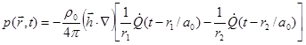
is zero. Their difference is 2![]() . According to (28),
the sound pressure from the two sources is:
. According to (28),
the sound pressure from the two sources is:
 .
(41)
.
(41)
![]() and
and ![]() are
respectively the distances from the observation point to the upper and lower
sphere centers:
are
respectively the distances from the observation point to the upper and lower
sphere centers:
![]() ,
,
![]() . (42)
. (42)
As ![]() we keep amplitude of
we keep amplitude of ![]() constant, then from
Eqs.(41) and (29),
constant, then from
Eqs.(41) and (29),
 ,
,
![]() . (43)
. (43)
The radial velocity can be obtained by:
![]() .
(44)
.
(44)
From
(43) and (44) we can see the ![]() dependence of the
sound field. The sound field has two lobes with strongest sound in the z
direction. The two lobes have the same magnitude but 1800 out of
phase. The force of the sphere acting on the medium is in z direction:
dependence of the
sound field. The sound field has two lobes with strongest sound in the z
direction. The two lobes have the same magnitude but 1800 out of
phase. The force of the sphere acting on the medium is in z direction:
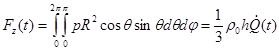 .
(45)
.
(45)
As ![]() , Eq.(43) becomes:
, Eq.(43) becomes:
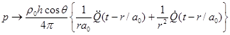 ,
,
![]() . (46)
. (46)
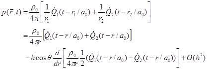
Compared
with the monopole solution (32), (46) shows the superposed sound field of two
monopoles with opposite strengths. This is called a dipole. Its strength is ![]() . To examine the physical meaning of the
dipole sound field (46), we expand the volume source at
. To examine the physical meaning of the
dipole sound field (46), we expand the volume source at ![]() for
small h:
for
small h:
 .
(47)
.
(47)
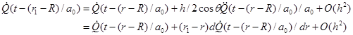
(Note:
![]() .) The source at
.) The source at ![]() can
be assumed to be at
can
be assumed to be at ![]() plus a correction. The
correction is due to the change of distance
plus a correction. The
correction is due to the change of distance ![]() and
the change of the retarded time
and
the change of the retarded time ![]() when the source is
repositioned. Applies the similar expansion to the source at
when the source is
repositioned. Applies the similar expansion to the source at ![]() . If we ignore the difference of
. If we ignore the difference of ![]() in
amplitude (
in
amplitude (![]() ), the sum of the two sources gives the
first term in (46). This term represents the sound source due to the difference
of the retarded time of the two sources.
), the sum of the two sources gives the
first term in (46). This term represents the sound source due to the difference
of the retarded time of the two sources.
On
the other hand, if we ignore the difference of the retarded time and
concentrate on the difference in ![]() , then we obtain the
second term of solution (46). This term is small in the farfield. In the
farfield the sound is mainly generated by the retarded time effect of the two
monopoles.
, then we obtain the
second term of solution (46). This term is small in the farfield. In the
farfield the sound is mainly generated by the retarded time effect of the two
monopoles.
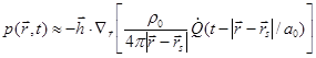
We can rewrite solution (46) in the form with the spatial derivative:
![]() .
(48)
.
(48)
The
spatial derivative is on the field coordinate, not the source coordinate. Because
of the retardation of the sound propagation from the source to the observer, the
sound field at observation time t has a spatial distribution, ![]() . The gradient of this spatial
distribution at the observation point in the direction of the dipole determines
the sound pressure at this point. The gradient includes two effects: the
retarded time difference and the propagation distance in amplitude. In the far field,
the retarded time effect is dominant; therefore one may take
. The gradient of this spatial
distribution at the observation point in the direction of the dipole determines
the sound pressure at this point. The gradient includes two effects: the
retarded time difference and the propagation distance in amplitude. In the far field,
the retarded time effect is dominant; therefore one may take ![]() out of the spatial derivative in (48).
out of the spatial derivative in (48).
In
terms of ![]() , the wave solution for the dipole is:
, the wave solution for the dipole is:
![]() ,
,
![]() . (49)
. (49)
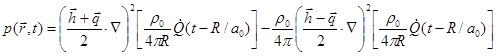
Solution (46) can also be directly
derived by performing the Taylor expansion on monopole solution (32). To
generalize the solution, suppose the dipole is situated at ![]() with the separation vector
with the separation vector ![]() , then,
, then,
 ,
(50)
,
(50)
![]() ,
, ![]() ,
, ![]() ,
, ![]() .
.
To first order Taylor expansion, we have:
 .
(51)
.
(51)
In Cartesian coordinates, the solution has this form:
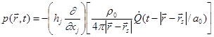 .
(52)
.
(52)
(51) and (52) are just generalized (48). The sound at the observation point is determined by the gradient of the monopole sound field in the direction of the dipole.
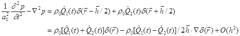
To
obtain the inhomogeneous wave equation for the dipole, one may attempt to
integrate ![]() over a sphere centered at the source as
in the monopole case. But the integration is zero since there is no net flow
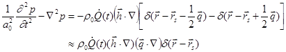
from the two monopoles. The correct way is to begin with the inhomogeneous wave
equation for monopole (37):
over a sphere centered at the source as
in the monopole case. But the integration is zero since there is no net flow
from the two monopoles. The correct way is to begin with the inhomogeneous wave
equation for monopole (37):
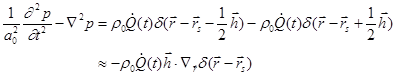 [HJ5] . (53)
Quadrupole (Momentum Flux Fluctuation)
Consider
two dipoles with the same strength ![]() but in opposite
directions. The distance between the two dipoles is
but in opposite
directions. The distance between the two dipoles is ![]() centered at
centered at ![]() as in Fig.3. According to (51), the
superposed sound pressure is:
as in Fig.3. According to (51), the
superposed sound pressure is:
 ,
(54)
,
(54)
![]() ,
, ![]() .
.
 |
Fig.3, A quadrupole.
To first order, the Taylor expansion of (54) is:
![]() ,
,
![]() . (55)
. (55)
In Cartesian coordinates, we can rewrite the solution as:
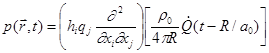 .
(56)
.
(56)
![]() and
and ![]() can
be in any direction. There are two special cases. If
can
be in any direction. There are two special cases. If ![]() and
and ![]() are parallel, the quadrupole
is longitudinal. A longitudinal quadrupole has two lobes in sound field.
Compared with a dipole, the two lobes from a longitudinal quadrupole are in
phase instead of out of phase. If
are parallel, the quadrupole
is longitudinal. A longitudinal quadrupole has two lobes in sound field.
Compared with a dipole, the two lobes from a longitudinal quadrupole are in
phase instead of out of phase. If ![]() and
and ![]() are perpendicular, the quadrupole is
lateral. There are four lobes in the sound field of a quadrupole.
are perpendicular, the quadrupole is
lateral. There are four lobes in the sound field of a quadrupole.
(55) can be rewrite to:
 .
(57)
.
(57)
Any quadrupole can be decomposed into two longitudinal quadrupoles. Longitudinal quadrupole is the basic type of all quadrupoles.
The inhomogeneous equation for a quadrupole is:
 .
(58)
.
(58)
In summary, any sound sources can be represented by superposition of monopoles. When monopoles are close to each other, models such as dipoles or quadrupoles are more appropriate. A quadrupole can always be separated into two longitudinal quadrupoles. Longitudinal quadrupole is the basic type of quadrupoles.
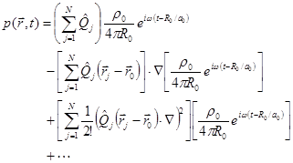
Multipole Expansions
Dipole is composed of two monopoles with equal strength but opposite signs, while a quadrupole is composed of four monopoles with equal strength but opposite signs. Monopole, dipole, quadrupole, etc., are the basic types of sound sources. If a source region is compact compared to the sound wavelengths, any source can be represented by the sum of these basic sources.
Let’s
begin with the sound field from two monopoles: one with strength![]() at
at ![]() and
the other with
and
the other with ![]() at
at ![]() .
According to (34), the total sound pressure is:
.
According to (34), the total sound pressure is:
 .
(59)
.
(59)
To
order of ![]() , the acoustic field is generated by a
monopole with strength
, the acoustic field is generated by a
monopole with strength![]() at their geometric center, and
a dipole with strength
at their geometric center, and
a dipole with strength ![]() . According to (37),
the inhomogeneous equation is:
. According to (37),
the inhomogeneous equation is:
 .
(60)
.
(60)
Suppose
there are N monopoles with strength ![]() at
at ![]() ,
, ![]() The
total sound pressure is:
The
total sound pressure is:
![]() ,
,
![]() . (61)
. (61)
Assume
the source region is small in all dimensions compared with the sound wave length,
and ![]() is the geometric center of the source
region. The sound pressure from the j-th monopole can be expanded about
is the geometric center of the source
region. The sound pressure from the j-th monopole can be expanded about ![]() :
:
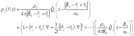 .
(62)
.
(62)
![]() .
.
Therefore the total sound pressure from all the monopoles is:
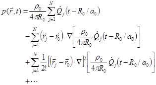 .
(63)
.
(63)
To
the zero-th order, the N monopoles can be represented by one monopole
with the total strength of all the monopoles. The dipoles seem not having an
equivalent dipole as in (60), where ![]() can be chosen in the
middle of the two monopoles. If all the monopoles oscillate at the same
frequency
can be chosen in the
middle of the two monopoles. If all the monopoles oscillate at the same
frequency ![]() ,
, ![]() ,
then,
,
then,
 .
(64)
.
(64)
Then the sound sources can be represented by one monopole, one dipole, and one quadrupole, etc. The equivalent monopole has the strength of the sum of all the monopoles. The dipole is in a direction of the vector sum of all the monopoles.
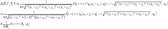
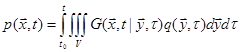
Green’s Function in Three Dimensional Open Space with No Flow
We have discussed the monopole and its high order derivatives. There are three types of sound sources in a flow: volume fluctuation, force, and viscous stress oscillation. They can be respectively modeled as monopoles, dipoles, and quadrupoles. Since high order poles can be constructed by monopoles, it is essential to solve the acoustic field of a monopole.
The
solution to the acoustic wave equation of a monopole with unit strength is
called the Green’s function[56].
Setting source strength per unit volume ![]() , a
pulse with unit strength emitting sound at
, a
pulse with unit strength emitting sound at ![]() , in the
inhomogeneous acoustics equation (37) and its solution (34), we have:
, in the
inhomogeneous acoustics equation (37) and its solution (34), we have:
![]() ,
(65)
,
(65)
![]() .
(66)
.
(66)
![]() is the Green’s function in a stationary
medium in the open space[57].
It represents the sound at the observation point
is the Green’s function in a stationary
medium in the open space[57].
It represents the sound at the observation point ![]() and
time t generated by a pulse at source point
and
time t generated by a pulse at source point ![]() released
at time
released
at time ![]() . The Green’s function in Eq.(66) is in
Cartesian coordinates. Green’s functions in cylindrical coordinates and in
spherical coordinates are also useful in applications and will be discussed
later. Operator
. The Green’s function in Eq.(66) is in
Cartesian coordinates. Green’s functions in cylindrical coordinates and in
spherical coordinates are also useful in applications and will be discussed
later. Operator ![]() has a subscript
has a subscript ![]() to explicitly indicate that the left
side of the equation is operated on the observation coordinate
to explicitly indicate that the left
side of the equation is operated on the observation coordinate ![]() . The Green’s function is often written
as
. The Green’s function is often written
as ![]() to explicitly indicate the field
(observer) coordinates and time and the source coordinates and emitting time.
This is very important in the following context.
to explicitly indicate the field
(observer) coordinates and time and the source coordinates and emitting time.
This is very important in the following context.
As ![]() , one obtains the three-dimensional
Laplacian equation and its Green’s function:
, one obtains the three-dimensional
Laplacian equation and its Green’s function:
![]() ,
(67)
,
(67)
![]() .
(68)
.
(68)
If
the medium moves at constant velocity ![]() , G
satisfies the more general inhomogeneous wave equation:
, G
satisfies the more general inhomogeneous wave equation:
![]() .
(69)(70)
.
(69)(70)
Obviously the Green’s function satisfying (70) is different from (66).
The Green’s function has three important properties (Rienstra2006 for proof):
(1)Causality: there is no sound before the source energy is released:
![]() ,
,
![]() , when
, when ![]() .
(71)
.
(71)
(2)Reciprocity:
![]() .
(72)
.
(72)
In this particular case (uniform medium), the Green function and its adjoint are the same function. It is self-adjoint, or symmetric. In general, the adjoint Green function is different from its original:
![]() ,
(73)
,
(73)
such as in the shear flow in Tam& Auriault1988.
![]() .
(74)
.
(74)
(4)![]() is singular with order
is singular with order ![]() at the source point.
at the source point.
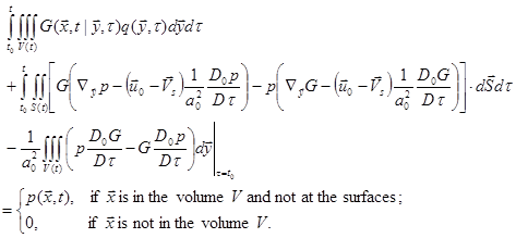
Integral Representation of Acoustic Equation: Kirchhoff’s Formula
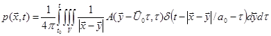
In the previous sections we have discussed the simple sources and the Green’s functions. The sound field from continuously distributed monopoles was briefly mentioned in Eq.(38) and (39). Here we will study distributed sources in more details.
Suppose we have a continuously
distributed source field ![]() in the moving medium.
The inhomogeneous acoustic wave equation is [ref.(13)&(38)]:
in the moving medium.
The inhomogeneous acoustic wave equation is [ref.(13)&(38)]:
![]() ,
or, (75)
,
or, (75)
![]() .
(76)
.
(76)
With
the Green’s function, the partial differential acoustic wave equation can be
transformed into an integral acoustic wave equation. The integration will be
operated on source coordinate ![]() and time
and time ![]() . The Green’s function satisfying (74)
instead of Eq.(70), will be used.
. The Green’s function satisfying (74)
instead of Eq.(70), will be used.
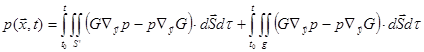
As
in Fig.1, control volume ![]() is bounded by surfaces
is bounded by surfaces
![]() , including inner surface
, including inner surface ![]() and outer surface
and outer surface ![]() . The surfaces can be arbitrary, where no
boundary conditions are enforced. Subtract Eq.(74) multiplied by p from
Eq.(76) multiplied by G, and integrate this equation over volume V from
time
. The surfaces can be arbitrary, where no
boundary conditions are enforced. Subtract Eq.(74) multiplied by p from
Eq.(76) multiplied by G, and integrate this equation over volume V from
time ![]() to t+ (t+ means inclusive
of t):
to t+ (t+ means inclusive
of t):
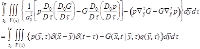 .
(77)
.
(77)
According to Green’s Second Identity:
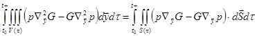 .
(78)
.
(78)
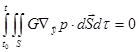
Sound
pressure p was chosen as the acoustic variable in Eqs.(75)&(76). p
is a single-valued function of position no matter if the region is
singly-connected or multiply-connected. If velocity potential ![]() is chosen as the acoustic variable, one concern
is that
is chosen as the acoustic variable, one concern
is that ![]() is single-valued only in a
singly-connected region. If the region is multiply-connected, artificial
barrier(s)
is single-valued only in a
singly-connected region. If the region is multiply-connected, artificial
barrier(s) ![]() should be inserted to make the region
singly-connected as in Fig.(2), and the surface integration in (78) should
include
should be inserted to make the region
singly-connected as in Fig.(2), and the surface integration in (78) should
include ![]() . However, the normal direction on the
two sides of the surface have opposite directions; the integration on the
barrier is zero. Therefore equation (78) applies for
. However, the normal direction on the
two sides of the surface have opposite directions; the integration on the
barrier is zero. Therefore equation (78) applies for ![]() as
well.
as
well.
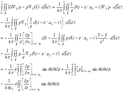
To
integrate ![]() in (77), we begin with the simplest case.
in (77), we begin with the simplest case.
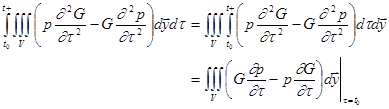
Stationary Control Volume in Stationary Medium
Consider a stationary control volume V
(relative to the observer) without mean flow, i.e., ![]() . Since V doesn’t vary with time,
the integration order can be exchanged:
. Since V doesn’t vary with time,
the integration order can be exchanged:
 .
.
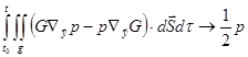
The integration
at ![]() is zero, required by the causality of
the Green’s function (71). Then we obtain the famous Kirchhoff’s formula in
stationary volume V without mean flow:
is zero, required by the causality of
the Green’s function (71). Then we obtain the famous Kirchhoff’s formula in
stationary volume V without mean flow:
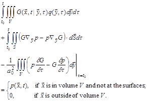 (79)
(79)
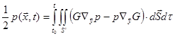
The Kirchhoff’s formula,
also called the Kirchhoff-Helmholtz Integral Theorem,
was first published in 1882. Although the formula is
presented on sound pressure, it holds for any other
acoustic variables. The first term on the left side is the sound field from the
distributed sources in the volume as if there were no
surfaces ![]() and
and ![]() . In
this case Green’s function (66) applies, and the Kirchhoff’s formula reduces to
(39) that was based on the principal of superposition.
The second term on the left side of (79) represents the effect of the (physical
boundary) surfaces on the sound field (refraction,
reflection, etc.), or the contribution of the sources from outside of
the surfaces. The last term on the left side is the effect of
the initial condition, which is zero if no sound exists initially. If
. In
this case Green’s function (66) applies, and the Kirchhoff’s formula reduces to
(39) that was based on the principal of superposition.
The second term on the left side of (79) represents the effect of the (physical
boundary) surfaces on the sound field (refraction,
reflection, etc.), or the contribution of the sources from outside of
the surfaces. The last term on the left side is the effect of
the initial condition, which is zero if no sound exists initially. If ![]() is on the surface, the volume integral
about the Delta function in (77) is undefined. A limit
analysis on (79) will be performed to derive a formula applicable for
is on the surface, the volume integral
about the Delta function in (77) is undefined. A limit
analysis on (79) will be performed to derive a formula applicable for ![]() on the surface.
on the surface.
The partial differential equation (76)
describes the relationship of a source and the sound near
it. On the other hand, Kirchhoff’s formula (79) connects the
source region to its far field sound field. It incorporates in a single equation the effects of the sources, the physical boundary or arbitrary permeable surfaces,
and the initial conditions. Generally the Kirchhoff’s formula is not a
solution. There are unknowns (p and ![]() ) in
the volume integral and in the surface integral in
(77). According to the solution uniqueness theorem, p and
) in
the volume integral and in the surface integral in
(77). According to the solution uniqueness theorem, p and ![]() cannot be prescribed independently on the
surfaces. One must be solved when the other is prescribed.
cannot be prescribed independently on the
surfaces. One must be solved when the other is prescribed.
Stationary Control Volume with Uniform Mean Flow
There are two ways to include a uniform
mean flow ![]() into the Kirchhoff’s formula. The first
is to follow the same procedure as for (79) (Goldstein1976). Note
into the Kirchhoff’s formula. The first
is to follow the same procedure as for (79) (Goldstein1976). Note
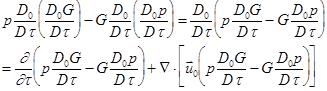 .
.
We have the Kirchhoff's formula for a stationary volume in a uniform mean flow:
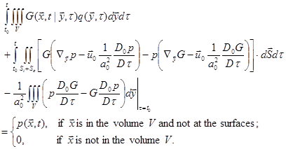 .
(80)
.
(80)
Note the extra terms in the surface integral compared to the no-flow Kirchhoff formula Eq.(79).
The second
method is to make use of the linear transformations of the coordinates.
Without loss of generality, we establish a coordinate with the ![]() -axis parallel to the mean flow, then
wave equation Eq.(75) is:
-axis parallel to the mean flow, then
wave equation Eq.(75) is:
![]() .
(81)
.
(81)
The simplest linear transformation is the Galilean transformation:
![]() ,
, ![]() ,
, ![]() ,
, ![]() .
(82)
.
(82)
With (82), (81) can be transformed to an equation in a stationary flow. All the analyses for the stationary medium apply. However, the property of the source/observer changes after the transformation. A stationary source in the coordinate system moves in the other coordinate system. The Lorentz-type transformation can be used to avoid it:
![]() ,
,
![]() ,
, ![]() , and
, and ![]() [GE8] , (83)
[GE8] , (83)
where ![]() ,
, ![]() . In this system, the dimension in
. In this system, the dimension in ![]() direction is dilated in a subsonic flow,
while the time is compressed and shifted. The amount of the time shift varies
with
direction is dilated in a subsonic flow,
while the time is compressed and shifted. The amount of the time shift varies
with ![]() . With this transformation, acoustic
equation (75) and the Green’s function equation become:
. With this transformation, acoustic
equation (75) and the Green’s function equation become:
![]() ,
(84)
,
(84)
![]() .
(85)
.
(85)
[Note:
![]() .] Acoustic equation (84) has the same
form as in a stationary medium, and the property of the source/observer doesn’t
change. Eq.(84) is now widely used in applications. (Morino)
.] Acoustic equation (84) has the same
form as in a stationary medium, and the property of the source/observer doesn’t
change. Eq.(84) is now widely used in applications. (Morino)
Transformation (83) is also called the Prandtl-Glauert Transformation, since the acoustic equation is reduced to the Prandtl-Glauert equation for compressible steady flows:
![]() .
.
Sometimes it is referred to as the Karman-Tsian Transformation.
Moving Control Volume with Uniform Mean Flow
Suppose
control surfaces ![]() moves with time. According to the
Leibniz’s Rule,
moves with time. According to the
Leibniz’s Rule,
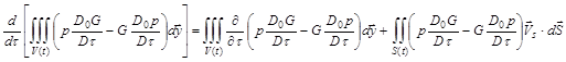
where
![]() is the moving velocity of the surface. Then
we have
is the moving velocity of the surface. Then
we have
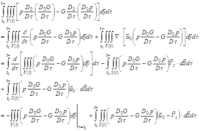
The Kirchhoff's formula for moving surfaces in a mean flow is
 (86)
(86)
This formula reduces to (79) or (80) without mean flow/moving surfaces. It is for general sources. To apply it for sources from flow in aeroacoustics, modifications/derivations are needed, such as Goldstein’s version, and the FW-H equation.
Applications of Kirchhoff’s Formulas
As we have mentioned, the Kirchhoff's formulas are the integral representations of the differential acoustic equations. Generally they are not the solutions. There is unknown variable in the surface integral of (79), (80) and (86): the surface integration is coupled with the sound field. The volume integration may also include the unknown variable if there is strong interaction between the source and the sound.
If there is no object in a stationary
medium and the sound has no back effect on its source ![]() , (79) reduces to:
, (79) reduces to:
 . (87)
In this case the Kirchhoff's formula is the solution. The sound field can be calculated by this formula using the open-space Green’s function (66) in the Cartesian coordinates in the open space. An example is the jet noise prediction. Noise from turbulence is modeled by the Lighthill Acoustic Analogy. The Lighthill stress is assumed known and the sound it generates assumes no back effect.
In
some situations, the coupling of the source and its generated sound on the
surfaces can be eliminated. If the surface is rigid, the non-penetration boundary
condition (![]() ) must be satisfied. Then
) must be satisfied. Then
 .
.
If the
Green’s function also satisfies the non-penetration boundary condition at the
surface (![]() ), then
), then
 .
.
Eq. (79) reduces to Eq.(87): the surface coupling is eliminated and Eq.(87) is the solution. But the Green’s function in Eq.(87) must satisfy the boundary condition at the surface. Check out Morse&Ingard1968, p. 500 for how to develop the Green’s function in a duct using the normal modes. Check out Howe1998: p.61, p.65 for the compact Green’s function which gives the leading order terms for the sound produced by sources near a solid body.
In general, it is difficult to find a Green’s function satisfying the boundary condition at the surfaces. If there is no volume source in a stationary medium, Eq.(79) reduces to:
 .
(88)
.
(88)
The
surface has two possible effects on the sound field. One is the diffraction: the
sound propagates towards the surface and is diffracted. The other is the object
surface acts as a sound source. No matter which type of effects, given p, ![]() (and
(and ![]() when there is mean flow) on the
body surface, the sound field can be calculated from Eq.(88). However, according to the solution uniqueness
theorem, to render a unique solution, only one of p and
when there is mean flow) on the
body surface, the sound field can be calculated from Eq.(88). However, according to the solution uniqueness
theorem, to render a unique solution, only one of p and ![]() , or a
linear combination of the two, can be prescribed on any part of the
surface. They cannot be
prescribed simultaneously. When one is prescribed, the other has to be solved. Therefore
either p or
, or a
linear combination of the two, can be prescribed on any part of the
surface. They cannot be
prescribed simultaneously. When one is prescribed, the other has to be solved. Therefore
either p or ![]() on the surface is an unknown
and needs to be solved.
on the surface is an unknown
and needs to be solved.
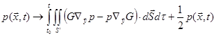
To solve the integral equation
(88), let's put the observation point ![]() on the surface as in Fig.4a. When
the source point approaches the observation point
on the surface as in Fig.4a. When
the source point approaches the observation point ![]() , the Green’s
function is singular. We will show the integral remains finite and is the sum
of the principal value of the integration and
, the Green’s
function is singular. We will show the integral remains finite and is the sum
of the principal value of the integration and ![]() .
.
a b
Fig.4, Observer on the surface.
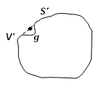
First
we deform the surface near the observer as in Fig.4b. The surface near the
observer is pushed into the object to form two new surfaces: S’and g.(
Ang2007) S’ is the original surface S excluding a small round
surface with radius ![]() . g is a half sphere
surface with radius
. g is a half sphere
surface with radius ![]() . The observer is in the new
volume V’ so Eq.(88) applies:
. The observer is in the new
volume V’ so Eq.(88) applies:
 .
(89)
.
(89)
Applying the free-space Green’s function (66), the second integral in (89) is:
 .
.
Suppose
the observer lies on a smooth part of S where ![]() is
smooth. As
is
smooth. As ![]() ,
,
 .
.
Plugging it into (89), we have,
 as
as
![]() . (90)
. (90)
The integral is over the original
surface S excluding the singular point (the observer). It is called the principal
integral. This shows the integral over S is the sum of its principal
value and ![]() . Eq.(90) is then simply:
. Eq.(90) is then simply:
 ,
,
![]() on S. (91)
on S. (91)
This is the boundary surface integral equation on sound pressure. (Crighton, et.al.1992, pp287-291, Pierce1989, p.182) After it is solved, the sound field can be computed from (88). The surface can be discretized so Eq.(91) is solved numerically. This is the boundary element method (BEM ). (Long-BEM.pdf, BEM2005.pdf)
If the inner surface is smooth, a model without circulation applies. In this model, the lift on the body is zero. If the surface has sharp edges, such as in an airfoil, the model without circulation will give singularity at sharp edges. In this case, the Kutta condition must be enforced to remove the singularity, which is equivalent to add circulation and lift to the medium and the body.
Other methods include CFD or CAA methods. One example is the sound from a jet. An artificial surface can be put around the jet, far enough so that the linear acoustic equation holds outside the surface. The flow field within the surface is known from other methods, such as experiment or numerical solutions.
Sound Field from Moving Sources
In
this section we will use Kirchhoff’s formula (87) to investigate the effect of moving
sources in an open space. The Green’s function for a stationary source in a
stationary medium in the Cartesian system, (66), is used in the analysis. A
stationary source oscillates but its time averaged position ![]() doesn’t move.
doesn’t move.
Sound Field from Moving Sources with Constant Velocity
The
simplest case is all the sources move with constant velocity ![]() . Establish a frame
. Establish a frame ![]() moving with the sources. The moving
frame is chosen to coincide with the fixed frame
moving with the sources. The moving
frame is chosen to coincide with the fixed frame ![]() at
at ![]() :
: ![]() . At
time
. At
time ![]() the coordinate of the source position in
the fixed frame is
the coordinate of the source position in
the fixed frame is
![]() .
(92)
.
(92)
Suppose
the strength of the source observed in the moving frame is ![]() . To facilitate the explanation, we
assume all the sources oscillate at the same angular frequency
. To facilitate the explanation, we
assume all the sources oscillate at the same angular frequency ![]() (constant-frequency assumption), while
their strengths vary with position, i.e.,
(constant-frequency assumption), while
their strengths vary with position, i.e.,
![]() .
(93)
.
(93)
To apply Green’s function (66), the source must be defined in the fixed frame:
![]() .
(94)
.
(94)
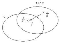
Fig.5, Effect of a moving source.
Examining
the source in Eq.(94) at ![]() in the fixed frame, one
may find it not only oscillates at
in the fixed frame, one
may find it not only oscillates at ![]() as in
as in ![]() , but its amplitude also varies as in
, but its amplitude also varies as in ![]() . Expression (94) formally separates the two
effects of the source: the oscillation and the convection. The physical meaning
can be explained by Fig.5. At time
. Expression (94) formally separates the two
effects of the source: the oscillation and the convection. The physical meaning
can be explained by Fig.5. At time ![]() the source is in the
elliptic region shown in the figure. Let’s observe the point marked by
the source is in the
elliptic region shown in the figure. Let’s observe the point marked by ![]() . Its coordinates in the fixed and moving
frames are
. Its coordinates in the fixed and moving
frames are ![]() and
and ![]() respectively.
Short time
respectively.
Short time ![]() later, the source region and the marked
point move by distance
later, the source region and the marked
point move by distance ![]() to a new position. But the
fixed observation point at
to a new position. But the
fixed observation point at ![]() in the moving frame
moves by distance
in the moving frame
moves by distance ![]() . At
. At ![]() the
amplitude of the source is
the
amplitude of the source is ![]() . It varies only when
. It varies only when ![]() is not uniform. The sound source in the
fixed frame is time dependent even it is steady (
is not uniform. The sound source in the
fixed frame is time dependent even it is steady (![]() ) in
the moving frame when it is nonuniform.
) in
the moving frame when it is nonuniform.
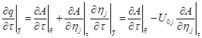
To
generate the sound, the source strength in the fixed frame must vary with time.
It is useful to investigate the time variation rate of the source at a fixed
point. The source strength observed at ![]() not
only varies with
not
only varies with ![]() as the source oscillates, but
also varies due to the source motion as shown by the first argument (
as the source oscillates, but
also varies due to the source motion as shown by the first argument (![]() ) of
) of ![]() in Eq.(94),
therefore,
in Eq.(94),
therefore,
 .
(95)
.
(95)
The
time changing rates of a quantity in the two frames are different: ![]() . Conventionally we denote the time rate
. Conventionally we denote the time rate ![]() observed in the fixed frame as
observed in the fixed frame as ![]() , and the time rate
, and the time rate ![]() observed in the moving frame as
observed in the moving frame as ![]() . Then,
. Then,
![]() .
(96)
.
(96)
![]() represents the source oscillation.
represents the source oscillation. ![]() is the source motion effect. The difference
between
is the source motion effect. The difference
between ![]() and
and ![]() is
the source motion effect. It can be neglected only when all of the three
conditions are satisfied: (1)source oscillation (
is
the source motion effect. It can be neglected only when all of the three
conditions are satisfied: (1)source oscillation (![]() ) is
not small; (2)the source moves slowly (
) is
not small; (2)the source moves slowly (![]() ); and
(3)the source strength is fairly uniform (
); and
(3)the source strength is fairly uniform (![]() ). If
a source is steady in the moving frame, such as the steady force on a rotating
blade, the first condition is not met. Since the source is on the blade surfaces,
its spatial distribution is highly nonuniform, therefore neither the 3rd
condition is satisfied. A steady force generates no sound if it doesn’t move.
The moving effect is the only sound generation mechanism in this case. It
shouldn’t be ignored under any circumstances in turbomachinery noise analyses.
). If
a source is steady in the moving frame, such as the steady force on a rotating
blade, the first condition is not met. Since the source is on the blade surfaces,
its spatial distribution is highly nonuniform, therefore neither the 3rd
condition is satisfied. A steady force generates no sound if it doesn’t move.
The moving effect is the only sound generation mechanism in this case. It
shouldn’t be ignored under any circumstances in turbomachinery noise analyses.
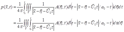
The effect of the moving source is now examined. Substituting source strength (94) and Green function (66) into the Kirchhoff’s formula (87), we have:
 .
(97)
.
(97)
Volume V includes all the sources
in the fixed frame. It occupies the whole space and is
not a function of time. The first argument in the source strength (![]() ) reflects the effect of source motion.
To express this effect explicitly, we may convert the
spatial integral from the fixed frame
) reflects the effect of source motion.
To express this effect explicitly, we may convert the
spatial integral from the fixed frame ![]() to the
moving frame
to the
moving frame ![]() :
:
 , (98)
The integration order can be changed in the last step since the whole space V is not a function of time.
For the
two functions ![]() and
and ![]() ,
we have
,
we have
![]() .
(99)
.
(99)
![]() is the nth root of
is the nth root of ![]() , i.e.,
, i.e.,
![]() .
(100)
.
(100)
![]() is the source emitting time for the
sound reaching the observer at time t. If the source moving speed is
subsonic, there is only one root (n=1). If the speed is supersonic,
there are two roots (n=2). It is not straightforward to solve
is the source emitting time for the
sound reaching the observer at time t. If the source moving speed is
subsonic, there is only one root (n=1). If the speed is supersonic,
there are two roots (n=2). It is not straightforward to solve ![]() from (100) even for the simple case of
uniformly moving source. When the source doesn’t move,
from (100) even for the simple case of
uniformly moving source. When the source doesn’t move, ![]() is
the same retarded time as before.
is
the same retarded time as before.
Note
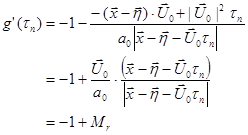 , (101)
![]() .
.
![]() is the angle between the source moving
direction and the source-observer vector at the emission time.
is the angle between the source moving
direction and the source-observer vector at the emission time. ![]() is the acoustic Mach number, or source
Mach number. It is not the actual Mach number since the source moving
velocity
is the acoustic Mach number, or source
Mach number. It is not the actual Mach number since the source moving
velocity ![]() is not the flow velocity.
is not the flow velocity. ![]() is the Mach number towards the observer.
is the Mach number towards the observer.
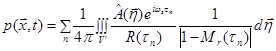
Substituting Eq.(99) and Eq.(101) into Eq.(98), the final expression for sound pressure from moving sources in time domain is:
![]() . [59]
(*5)(102)
. [59]
(*5)(102)
For a harmonic source,
 .
(*)
.
(*)
![]() is the distance between the observer and
the source at emission time
is the distance between the observer and
the source at emission time ![]() . Formally, the
sound field from a moving source is the sound field as if the source is
stationary divided by
. Formally, the
sound field from a moving source is the sound field as if the source is
stationary divided by ![]() . The motion has two major
effects. The first is the amplitude factor 1/
. The motion has two major
effects. The first is the amplitude factor 1/![]() . It
is solely due to the source motion, and generated when the spatial integration
over
. It
is solely due to the source motion, and generated when the spatial integration
over ![]() in the fixed frame is converted to that
over
in the fixed frame is converted to that
over ![]() in the moving frame. The complexity of
the spatial integration over
in the moving frame. The complexity of
the spatial integration over ![]() in Eq.(97) due to
in Eq.(97) due to ![]() is relieved in (102) since the first
argument in
is relieved in (102) since the first
argument in ![]() is no longer a function of time. However,
the complexity doesn’t disappear. It is just moved to the amplitude factor 1/
is no longer a function of time. However,
the complexity doesn’t disappear. It is just moved to the amplitude factor 1/![]() .
.
The
other major effect of motion is on the emission time ![]() ,
which affects amplitude factors 1/R and 1/
,
which affects amplitude factors 1/R and 1/![]() , and mostly importantly affects the
phase and the frequency.
, and mostly importantly affects the
phase and the frequency.
For
a steady source, ![]() ,
, ![]() ,
, ![]() . There is no sound since
. There is no sound since ![]() does not vary with time. On the other
hand, if the source moves, then
does not vary with time. On the other
hand, if the source moves, then ![]() and
and ![]() are time dependent and the sound is
generated.
are time dependent and the sound is
generated.
For
the harmonic source in the moving frame as in (93), if the source doesn’t move,
the sound amplitude at the observation point is ![]() . The
frequency in the sound field is the same as in the source:
. The
frequency in the sound field is the same as in the source: ![]() (
(![]() ). The
effects of the source motion on the sound amplitude and the phase are seemly
separated in (102). The sound amplitude is changed through
). The
effects of the source motion on the sound amplitude and the phase are seemly
separated in (102). The sound amplitude is changed through ![]() and
and ![]() . The
sound received by an observer in front of the source (
. The
sound received by an observer in front of the source (![]() )
is stronger than that received by an observer behind the source (
)
is stronger than that received by an observer behind the source (![]() ). On the other hand, the source motion
effect on frequency is through
). On the other hand, the source motion
effect on frequency is through ![]() . To show it, let’s
assume the source motion speed is subsonic and in the far field:
. To show it, let’s
assume the source motion speed is subsonic and in the far field:
![]() .
(103)
.
(103)
The retarded time is:
![]() .
(*5-1)(104)
.
(*5-1)(104)
According
to Eq.(102) the sound pressure has time factor ![]() . The
sound frequency measured in the fixed frame is
. The
sound frequency measured in the fixed frame is ![]() .
Time in the fixed frame, t, is compressed therefore its frequency increases
when the source moves towards the observer. This is the Doppler effect through
phase, and
.
Time in the fixed frame, t, is compressed therefore its frequency increases
when the source moves towards the observer. This is the Doppler effect through
phase, and ![]() is the Doppler factor. (When
is the Doppler factor. (When ![]() the Doppler factor and the sound field
become singular and special treatment is needed.)
the Doppler factor and the sound field
become singular and special treatment is needed.)
The observation
time is compressed in (104) which can be explained further from (100). Assume ![]() , then,
, then,
![]() .
.
Then,
![]() ,
,
![]() . (105)
. (105)
Because
of the source motion, ![]() and
and ![]() are
no longer equal, which has also been shown by (96). Changing rates of any
quantity in reception time and emission time are different.
are
no longer equal, which has also been shown by (96). Changing rates of any
quantity in reception time and emission time are different.
Exactly
speaking, frequency is the recurrence of an oscillation returns to the same
state. That requires the oscillation has constant amplitude. Mathematically the
Fourier transform of a signal gives Fourier components with constant
amplitudes. Therefore the variation of amplitude due to ![]() and
and
![]() in (102) also changes the frequency and
gives the Doppler effect. We may consider this as the Doppler effect
through amplitude. The variation of amplitude corresponds to Fourier components
at different frequencies. Therefore the effects of the source motion on sound
amplitude and phase are not exactly separated in (102).
in (102) also changes the frequency and
gives the Doppler effect. We may consider this as the Doppler effect
through amplitude. The variation of amplitude corresponds to Fourier components
at different frequencies. Therefore the effects of the source motion on sound
amplitude and phase are not exactly separated in (102).
The
sound field in (102) is the sum over the possible emission times ![]() from (100). From now on we will
omit this summation for convenience.
from (100). From now on we will
omit this summation for convenience.
Sound Field from Arbitrarily Moving Sources
All analyses for the sound field from uniformly moving sources are valid for arbitrarily moving sources except that
 .
(106)
.
(106)
Approximations
Solution (102) is concise and has clear physical meaning. It is the basis for developing numerical methods in time domain. Ref. to cht22.doc for details. It can hardly be directly used in frequency domain without any approximations.
Two
types of approximations are usually made. The first is on amplitude factor ![]() .
. ![]() when
when ![]() is small, such as in Eq.(12-43) in
Blake. However, this approximation can only be made when the other two of the
three conditions as discussed previously are met: (1) the source oscillation is
not small, and (2) the source strength is fairly uniform. Obviously this is not
the case in turbomachinery since sources on blade surfaces are strongly
discontinuous in space.
is small, such as in Eq.(12-43) in
Blake. However, this approximation can only be made when the other two of the
three conditions as discussed previously are met: (1) the source oscillation is
not small, and (2) the source strength is fairly uniform. Obviously this is not
the case in turbomachinery since sources on blade surfaces are strongly
discontinuous in space. ![]() appears when the
integration in the fixed frame is converted to the integration in the moving
frame. In time-domain methods integrations are implemented in the physical
domain. It is convenient to use the moving frame. Therefore
appears when the
integration in the fixed frame is converted to the integration in the moving
frame. In time-domain methods integrations are implemented in the physical
domain. It is convenient to use the moving frame. Therefore ![]() appears a lot in these methods. In
frequency domain methods, solutions are expressed in modes. Sources are coupled
with mode shapes, which can easily convert between the fixed and the moving
frames. Therefore a fixed frame is usually adopted in frequency domain methods
and handling of
appears a lot in these methods. In
frequency domain methods, solutions are expressed in modes. Sources are coupled
with mode shapes, which can easily convert between the fixed and the moving
frames. Therefore a fixed frame is usually adopted in frequency domain methods
and handling of ![]() is avoided.
is avoided.
The
second type of approximation is on the emission time and the distance. Most of
the complexity of moving source noise prediction comes from finding the
emission time ![]() in (100) from the reception
time t. This is not easy even for a source moving at constant velocity.
One way to get around it is to compute the sound field in source time
in (100) from the reception
time t. This is not easy even for a source moving at constant velocity.
One way to get around it is to compute the sound field in source time ![]() instead of reception time t.
t can be directly computed from
instead of reception time t.
t can be directly computed from ![]() by
(100). This strategy is applicable in time-domain numerical simulations. (Ref.
cht22.doc for time domain method) In analyses the reception time is preferred.
It is not avoidable to find the emission time.
by
(100). This strategy is applicable in time-domain numerical simulations. (Ref.
cht22.doc for time domain method) In analyses the reception time is preferred.
It is not avoidable to find the emission time.
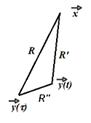
Fig.6, Approximation
of ![]() by
by ![]() for
finding the retarded time.
for
finding the retarded time.
Depending
on the conditions, there are two approximations for R and ![]() . In the far field, R can
be approximated by Eq.(103) and the emission time by (104). It is often used
for high-speed rotors. For a slowly moving source. the retarded time in
. In the far field, R can
be approximated by Eq.(103) and the emission time by (104). It is often used
for high-speed rotors. For a slowly moving source. the retarded time in ![]() in the phase is ignore and
in the phase is ignore and ![]() in Eq.(100) is replaced by
in Eq.(100) is replaced by ![]() shown in Fig.6:
shown in Fig.6:
![]() ,
,
from which the retarded time can be obtained readily:
![]() .
(107)
.
(107)
Note
![]() ,
, ![]() ,
,
![]() .
.
If ![]() , the error of the approximation is:
, the error of the approximation is:
![]() .
.
It is justified for slowly moving sources. This approximation is widely used in low speed turbomachinery noise analyses.
Another
approximation is often made on amplitude factor 1/![]() . In
the far field the moving effect on
. In
the far field the moving effect on ![]() is often ignored. A
constant R between the observer and the geometric center of the source
region can be used.
is often ignored. A
constant R between the observer and the geometric center of the source
region can be used.
Sound Field from Rotating Sources
In this section we will apply (102) in the investigation of sound field generated by rotating sources. It is convenient to use the cylindrical coordinates shown by Fig.7 in the frame moving with the sources:
![]() ,
(108)
,
(108)
and in the fixed frame:
![]() .
(109)
.
(109)
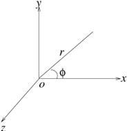
Fig.7, Cylindrical coordinates.
The
source rotates at angular speed ![]() on the
on the ![]() plane. The cylindrical coordinate
relation between the two frames is:
plane. The cylindrical coordinate
relation between the two frames is:
![]() .
(109)
.
(109)
Ignoring the moving effect in amplitude
Since the moving effect is ignored in the amplitude, this analysis only applies for source oscillating at high frequency in the moving frame.
The
sound pressure at observation point ![]() with cylindrical
coordinates
with cylindrical
coordinates ![]() can be evaluated by Eq.(102). The first
approximation we make is in the far field to approximate
can be evaluated by Eq.(102). The first
approximation we make is in the far field to approximate ![]() in the amplitude by
in the amplitude by ![]() . When the rotating speed is small (
. When the rotating speed is small (![]() ), it seems natural to neglect the moving
effect in the amplitude, i.e.,
), it seems natural to neglect the moving
effect in the amplitude, i.e., ![]() , as
in Blake sec.12.2.2. Then in the far field,
, as
in Blake sec.12.2.2. Then in the far field,
![]() .
(110)
.
(110)
With
![]() assumed,
assumed, ![]() in
the source phase may be approximated by
in
the source phase may be approximated by ![]() as shown
in Fig.6 so that the retarded time can be obtained from Eq.(107) in which
as shown
in Fig.6 so that the retarded time can be obtained from Eq.(107) in which
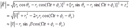 .
(111)
.
(111)
![]() is the angle between
is the angle between ![]() and the z-axis,
and the z-axis, ![]() .
.
For a
harmonic source in the moving frame: ![]() (change to (93)?),
(110) becomes:
(change to (93)?),
(110) becomes:
![]() ,
,
where
![]() .
.
![]() ,
, ![]() ,
,
is often used to expand a
plane wave as a sum of
cylindrical waves. (cf. Morse&Ingard1968, Eq.(1.2.9) at p.13). With this
expansion, variables about ![]() and
and ![]() in the sound pressure expression can be
separated and the sound pressure in cylindrical coordinates is:
in the sound pressure expression can be
separated and the sound pressure in cylindrical coordinates is:
![]() . (112)
. (112)
For
the single frequency ![]() observed in the
moving frame, there exist multiple frequencies in the fixed frame due to the
Doppler effect through phase:
observed in the
moving frame, there exist multiple frequencies in the fixed frame due to the
Doppler effect through phase: ![]() , integer
, integer ![]() . At each frequency
. At each frequency ![]() , there is a spinning mode pattern in the
circumferential direction with spinning mode number n.
, there is a spinning mode pattern in the
circumferential direction with spinning mode number n.
Once
the frequency and the amplitude of the source in the moving frame are known,
sound pressure can be computed from (112). If the source is steady in the
moving frame (![]() ), such as a steady force, no
sound is computed from this formula. This is due to the assumption of
), such as a steady force, no
sound is computed from this formula. This is due to the assumption of ![]() . Solution (112) only applies for sources
with high frequency oscillations. For steady sources in the moving frame,
effect of
. Solution (112) only applies for sources
with high frequency oscillations. For steady sources in the moving frame,
effect of ![]() must be retained.
must be retained.
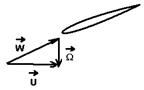
Fig.8, Airfoil subjected to incident flow.
Suppose a rotor with B blades
rotates in the wake of a stator with V vanes. To investigate the source
characteristics, let’s concentrate on one rotating blade as in Fig.8. The aerodynamics
of the flow over the blade depends primarily on the incident velocity ![]() :
:
![]() . (113)
. (113)
![]() is the upstream velocity in the fixed
frame,
is the upstream velocity in the fixed
frame, ![]() is the blade rotating
velocity. The source strength depends on
is the blade rotating
velocity. The source strength depends on ![]() and
its direction (angle of attack), therefore is a function of
and
its direction (angle of attack), therefore is a function of ![]() , the wake flow of the upstream stator.
In the fixed frame, the wake flow is periodic in
, the wake flow of the upstream stator.
In the fixed frame, the wake flow is periodic in ![]() with
period
with
period ![]() . It can be represented by this
Fourier series:
. It can be represented by this
Fourier series:
![]() . (114)
. (114)
In the rotating frame the wake becomes:
![]() . (115)
. (115)
Observed
at position ![]() in the moving frame, the
incident velocity oscillates with amplitude
in the moving frame, the
incident velocity oscillates with amplitude ![]() at
frequency
at
frequency
![]() (115-1)
(115-1)
when
the blade moves through the wake. The rotation of the rotor blade transforms
the flow spatial nonuniformity in the stator wake into time nonuniformity. Frequency
![]() of the source observed in the moving
frame is the stator blade passing frequency (BPF) and its harmonics,
depending on the rotation speed of the stator relative to the rotor and the number
of stator vanes, instead of the number of the rotor blades.
of the source observed in the moving
frame is the stator blade passing frequency (BPF) and its harmonics,
depending on the rotation speed of the stator relative to the rotor and the number
of stator vanes, instead of the number of the rotor blades.
The
blade at ![]() responds to the incident wake with
the source strength in a form similar to (115):
responds to the incident wake with
the source strength in a form similar to (115):
![]() . (116)
. (116)
The
Dirac delta function is to indicate that the sound source only exists when the
blade occupies the space. The B rotor blades are separated by ![]() . The sound source at the jth
blade is:
. The sound source at the jth
blade is:
![]() . (117)
. (117)
If we concentrate on the mth Fourier component of the wake in (115), the source is:
![]() , (118)
, (118)
![]() .
.
The corresponding sound pressure is
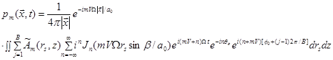 .
.
Since
![]() ,
,
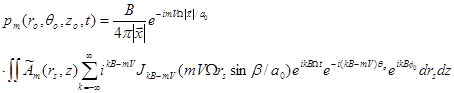 . (119)
This
result is similar to Eq.(12-14) of Blake. The sound frequencies observed in the
fixed frame are ![]() , the rotor
blade-passing frequency (BPF) and its harmonics. They depend on the rotation
speed of the rotor relative to the stator, and the number of rotor
blades. They are totally different from the source frequency
, the rotor
blade-passing frequency (BPF) and its harmonics. They depend on the rotation
speed of the rotor relative to the stator, and the number of rotor
blades. They are totally different from the source frequency ![]() , which is the stator blade-passing
frequency and its harmonics. Corresponding to each frequency
, which is the stator blade-passing
frequency and its harmonics. Corresponding to each frequency ![]() , there is a spinning mode in the
circumferential direction:
, there is a spinning mode in the
circumferential direction: ![]() . (Spinning
mode is defined positive if it propagates in positive
. (Spinning
mode is defined positive if it propagates in positive ![]() direction.) It can be showed that the
frequency at observer
direction.) It can be showed that the
frequency at observer ![]() is the difference
between the source frequency
is the difference
between the source frequency ![]() and the
spinning mode
and the
spinning mode ![]() rotating frequency
rotating frequency ![]() . This
is consistent with the fact that the time rate in the fixed frame is the
difference of the time rate in the moving frame and the changing rate due to
the source gradient:
. This
is consistent with the fact that the time rate in the fixed frame is the
difference of the time rate in the moving frame and the changing rate due to
the source gradient: ![]() . It is called the frequency scattering. The radiation
coefficient,
. It is called the frequency scattering. The radiation
coefficient, ![]() , is determined by the spinning
mode and the source frequency
, is determined by the spinning
mode and the source frequency ![]() .
.
For
a steady source in the rotating frame, ![]() ,
,
![]() is constant according to (119), i.e.,
no sound. The Doppler effect through amplitude, or
is constant according to (119), i.e.,
no sound. The Doppler effect through amplitude, or ![]() ,
was ignored when deriving (119). As we have mentioned, the source distribution
on the rotating blade surfaces is highly nonuniform in space. Effect of
,
was ignored when deriving (119). As we have mentioned, the source distribution
on the rotating blade surfaces is highly nonuniform in space. Effect of ![]() cannot be neglected even
cannot be neglected even ![]() is small.
is small.
Keeping the moving effect in amplitude
To keep the Doppler effect through amplitude, it is better to model the source directly in the fixed frame (Morse&Ingard1968, p.738). Then the source is stationary in the Kirchhoff integration.
In
the fixed coordinate the wake is Eq.(114).Suppose at time ![]() , a rotator blade occupies the space at
fixed point
, a rotator blade occupies the space at
fixed point ![]() . The source at the blade is
proportional to
. The source at the blade is
proportional to ![]() . Since the rotor is
rotating at speed
. Since the rotor is
rotating at speed ![]() , the occurrence
frequency of a blade at this location is
, the occurrence
frequency of a blade at this location is ![]() (rotor
BPF). The time factor is then
(rotor
BPF). The time factor is then ![]() . n is
the harmonic of the BPF. The same argument applies at another location except
that there is time lag
. n is
the harmonic of the BPF. The same argument applies at another location except
that there is time lag ![]() . Therefore the
correct time factor is
. Therefore the
correct time factor is ![]() , and the model of the
source strength is:
, and the model of the
source strength is:
![]() . (120)
. (120)
n
begins with 1 since n=0 corresponds to a steady source which generates
no sound. This expression reflects the source motion effect we discussed
previously. (It is produced by the source motion and the source strength
gradient?). The difference of the source models in the fixed frame (120) and in
the moving frame (117) is that in the fixed frame, the source is continuously
distributed with ![]() , while in the moving
frame it is discrete with
, while in the moving
frame it is discrete with ![]() as it exists
only when the blades occupy that position. In the fixed frame the source exists
at any point in the source region as the rotor rotates.
as it exists
only when the blades occupy that position. In the fixed frame the source exists
at any point in the source region as the rotor rotates.
Substituting source model (120) into the Kirchhoff formula (102), we obtain the sound pressure from the mth component of the wake:
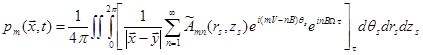 .
.
With the approximation (111) for slowly moving sources and the Jacobi-Anger expansion, the sound pressure is
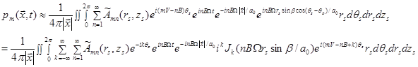
i.e.,
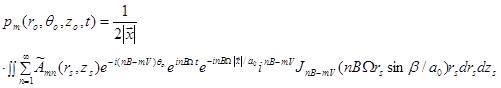 . (121)
This
is a rather different result from (119). It is the rotor blade passing
frequencies in ![]() instead of the
stator BPFs as in (119).
instead of the
stator BPFs as in (119).
The
sound frequencies are the rotor blade passing frequency and its harmonics: ![]() . The spinning (circumferential) mode of
the sound field is
. The spinning (circumferential) mode of
the sound field is ![]() , the difference of the
stator (wake) harmonic and the rotor harmonic, also called the Sofrin-Tyler
mode. For each frequency, i.e., fixed n, there are multiple spinning
modes for different m. For each spinning mode, the sound pressure is:
, the difference of the
stator (wake) harmonic and the rotor harmonic, also called the Sofrin-Tyler
mode. For each frequency, i.e., fixed n, there are multiple spinning
modes for different m. For each spinning mode, the sound pressure is:
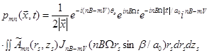 . (122)
The
circumferential period of the spinning mode is ![]() .
The rotation speed (phase speed) of the spinning mode is
.
The rotation speed (phase speed) of the spinning mode is ![]() .
.
Although the source (120) was modeled in the fixed frame to develop the solution, sometimes it is more convenient to determine the source in the rotating frame either numerically or theoretically. Substituting (109) into (120), the source in the rotating frame is:
![]() . (123)
. (123)
(123 vs.117?)
If
we solve the gust/blade interaction problem in frequency domain in the rotating
frame, we obtain the source strength ![]() with time
factor
with time
factor ![]() . It can be decomposed into
. It can be decomposed into ![]() according to this relationship:
according to this relationship:
![]() . (124)
. (124)
Once
![]() is determined, the sound pressure of
this spinning mode can be determined by the integration in the source region of
this source strength multiplied by weighting function
is determined, the sound pressure of
this spinning mode can be determined by the integration in the source region of
this source strength multiplied by weighting function ![]() .
. ![]() and
and
![]() in the weighting function reflect the
importance of the source location to the sound field. The source at larger
radius generates stronger sound. There is no sound along the axis (
in the weighting function reflect the
importance of the source location to the sound field. The source at larger
radius generates stronger sound. There is no sound along the axis (![]() ) except when
) except when ![]() .
This actually is the result of source motion effect. When
.
This actually is the result of source motion effect. When ![]() the sound arriving at the axis cancels
each other when the source rotates. On the other hand, when
the sound arriving at the axis cancels
each other when the source rotates. On the other hand, when ![]() , sound waves enforce each other, which
should be avoided to control the rotor noise. At some radial locations,
, sound waves enforce each other, which
should be avoided to control the rotor noise. At some radial locations, ![]() =0. This is also the effect of source
motion. When the source at one of these locations rotates, the sound is
cancelled as long as the observation point has angle
=0. This is also the effect of source
motion. When the source at one of these locations rotates, the sound is
cancelled as long as the observation point has angle ![]() .
.
Sound generated by two rotors
The similar analysis also applies for a wake generated by a front rotor instead of a stator. In the frame moving with the front rotor, the wake is:
![]() . (125)
. (125)
![]() is the circumferential angle in the
frame rotating with the front rotor. Suppose the front rotor rotates at speed
is the circumferential angle in the
frame rotating with the front rotor. Suppose the front rotor rotates at speed ![]() , then in the fixed frame the wake is:
, then in the fixed frame the wake is:
![]() . (126)
. (126)
In
the fixed frame, suppose at time ![]() an aft rotor
blade occupies the space at
an aft rotor
blade occupies the space at ![]() . Since a
blade passes this point at the aft rotor Blade Passing Frequency
. Since a
blade passes this point at the aft rotor Blade Passing Frequency ![]() , the source has time factor:
, the source has time factor:
![]() .
.
![]() is the time lag at a different
circumferential location. n is the harmonic of the aft rotor BPF. The
source strength is modeled as:
is the time lag at a different
circumferential location. n is the harmonic of the aft rotor BPF. The
source strength is modeled as:
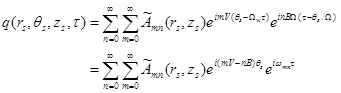 , (127)
Frequency
in the fixed frame is ![]() . Different from the
stator/rotor model (123), here n begins with 0.
. Different from the
stator/rotor model (123), here n begins with 0.
Substituting source model (127) into the Kirchhoff formula (102), making use of the approximation (111) and the Jacobi-Anger expansion, the sound pressure in the far-field is:
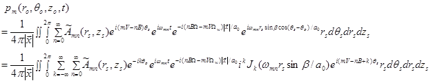 ,
,
i.e.,
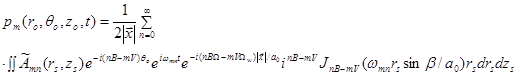 . (128)
This
solution reduces to (121) as ![]() . It reduces
to the solution of a front rotor interacting with a aft stator as
. It reduces
to the solution of a front rotor interacting with a aft stator as ![]() .
.
In
the stator/rotor case (121), there may be multiple spinning modes at one
frequency. Here for the rotor/rotor case, one spinning mode (m,n)
corresponds to only one frequency, vice versa. The sound field have
modes other than (m,n) at one specific frequency only when it is
scattered by nonuniformity such as splices in a duct during propagating process.
The frequency at observer ![]() is the difference
between the source frequency
is the difference
between the source frequency ![]() and the
spinning mode
and the
spinning mode ![]() rotating frequency
rotating frequency ![]() . This
is consistent with the fact that the time rate in the fixed frame is the
difference of the time rate in the moving frame and the changing rate due to
the source gradient:
. This
is consistent with the fact that the time rate in the fixed frame is the
difference of the time rate in the moving frame and the changing rate due to
the source gradient: ![]() . It is called the frequency scattering.
. It is called the frequency scattering.
Based
on solution (128), sound intensity of mode (m,n) depends on two factors:
(1) source strength ![]() , and (2) source
location as in radiation coefficient
, and (2) source
location as in radiation coefficient ![]() . Usually
the lower the spinning mode number
. Usually
the lower the spinning mode number ![]() , the higher
the radiation coefficient
, the higher
the radiation coefficient ![]() . If
. If ![]() is large,
is large, ![]() even
even
![]() is large. This mode is called 'cut-off'.
is large. This mode is called 'cut-off'.
![]() becomes important only when the
frequency increases to some level. Then the mode is 'cut-on'. (Blake1986,
Vol.2, p.882) This is how the 'cut-on' and 'cut-off' phenomenon is explained
when the Green's function in the Cartesian coordinates (66) is used. The
Green's function expressed in cylindrical coordinates will be given later. The
'cut-on' phenomena will be explained in a slightly different way.
becomes important only when the
frequency increases to some level. Then the mode is 'cut-on'. (Blake1986,
Vol.2, p.882) This is how the 'cut-on' and 'cut-off' phenomenon is explained
when the Green's function in the Cartesian coordinates (66) is used. The
Green's function expressed in cylindrical coordinates will be given later. The
'cut-on' phenomena will be explained in a slightly different way.
The
response of the aft rotor is roughly periodic in the circumferential direction,
i.e., ![]() is stronger when
is stronger when ![]() is close to B and its harmonics.
Therefore, based on B and V, we can estimate that, the mode whose
is close to B and its harmonics.
Therefore, based on B and V, we can estimate that, the mode whose
![]() is small and close to B and its
harmonics has stronger sound intensity. To control noise, B and V
must be selected carefully.
is small and close to B and its
harmonics has stronger sound intensity. To control noise, B and V
must be selected carefully.
As
an example, let’s assume ![]() and
and ![]() . For
. For ![]() ,
the spinning mode numbers are 12,2,-8,-18,…, when n=0,1,2,3,… The
spinning mode number (absolute value) closest to B is –8, therefore the
strong sound can be expected at mode (m,n)=(1,2). For
,
the spinning mode numbers are 12,2,-8,-18,…, when n=0,1,2,3,… The
spinning mode number (absolute value) closest to B is –8, therefore the
strong sound can be expected at mode (m,n)=(1,2). For ![]() , the spinning mode numbers are
24,14,4,-6,,… as n=0,1,2,3,… The spinning mode numbers (absolute value)
closer to B=10 are 4 and –6, therefore the strong sound can be expected
at mode (m,n)=(2,2) and (2,3). In this example, none of any combination
of m and n produces a spinning number equal to 10. V and B
are designed to avoid this happening.
, the spinning mode numbers are
24,14,4,-6,,… as n=0,1,2,3,… The spinning mode numbers (absolute value)
closer to B=10 are 4 and –6, therefore the strong sound can be expected
at mode (m,n)=(2,2) and (2,3). In this example, none of any combination
of m and n produces a spinning number equal to 10. V and B
are designed to avoid this happening.
Examining (121), we find no cutoff mechanism of the sound propagation in the free space. This is different from a rotor generating sound in a duct. In a duct only a limited number of modes can propagate. Other modes are evanescent. For the rotor-alone steady pressure generated sound, it propagates only when the tip speed reaches or exceeds supersonic. (Hubbard1995, p.167)
The source in the frame rotating with the aft rotor is:
![]() . (129)
. (129)
If
we solve the gust/blade interaction problem in frequency domain in the rotating
frame, we obtain the source strength ![]() with time
factor
with time
factor ![]() . It can be decomposed into
. It can be decomposed into ![]() according to this relationship:
according to this relationship:
![]() . (130)
. (130)
Once
![]() is determined, the sound pressure of
this spinning mode can be determined by Eq.(128).
is determined, the sound pressure of
this spinning mode can be determined by Eq.(128).
Green’s Functions in Cylindrical Coordinates in Open Space
When
we say the Green's function in cylindrical coordinates, we mean ![]() .
.
Green's function in cylindrical coordinates: Morse&Ingard, Eq.(7.3.15). It is derived from the Cartesian Green’s function using the Jacobi-Anger expansion.
General solution in cylindrical coordinates: Morse&Ingard, p.360
In application, the Green’s function in Cartesian coordinates is often used, and the Jacobi–Anger expansion is used to transfer it to the cylindrical coordinates when needed. It should give the same result as using the Green’s function in cylindrical coordinates directly.
J, Y: good for standing waves, therefore in ducts
H: good for propagating waves in open space
Spherical coordinate system: appropriate when the source region is concentrated in a small region of space (in all three dimensions)
Cylindrical coordinate system: appropriate when the source region is extended in one direction and concentrated in the other two.
Cartesian coordinate system: appropriate when the region extended in 2 dimensions.
Appropriate coordinate systems are also chosen based on the source integration when the source region is not compact. In this case the source integration is needed. Then appropriate coordinate system is chosen for the convenience of numerical integration
Green's function in spherical coordinates: Morse&Ingard, Eq.(7.2.31)
Green’s Functions in Two Dimensions
The Green’s functions in a three-dimensional stationary medium in open space are given by Eq.(66) in Cartesian coordinates and by ** in cylindrical coordinates. A point source in two dimensions can be modeled as a line source in three dimensions. Therefore the 2D Green’s function can be obtained by integrating along the line source. The 2D Green’s function can also be obtained by directly solving the 2D acoustic equation. The second approach is used in this section.
The non-homogeneous two-dimensional equation for the Green’s function is:
The
point source at ![]() oscillates at
circular frequency
oscillates at
circular frequency ![]() . The solution has the same
frequency so we can define:
. The solution has the same
frequency so we can define:
2D Green’s Function in Stationary Medium
We
first discuss the case ![]() . The solution is
axially symmetric. Polar coordinate (
. The solution is
axially symmetric. Polar coordinate (![]() ) is adopted:
) is adopted:
The axisymmetric equation in the polar coordinate system is:
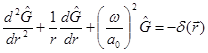 . (133)
The corresponding homogeneous equation of (133) (replacing the right hand side by 0) is the Bessel equation. Its general solution can be constructed by the two linearly independent Bessel functions:
![]() . (134)
. (134)
![]() and
and ![]() are
the zeroth order first and second kind of Bessel function respectively. A
and B are determined by boundary conditions at two radial locations.
Solution (134) represents standing waves such as in an annular duct
(cht16.doc). For open space we are discussing, (134) is not an appropriate
choice. Instead, we use the third kind of Bessel functions:
are
the zeroth order first and second kind of Bessel function respectively. A
and B are determined by boundary conditions at two radial locations.
Solution (134) represents standing waves such as in an annular duct
(cht16.doc). For open space we are discussing, (134) is not an appropriate
choice. Instead, we use the third kind of Bessel functions:
![]() and
and
![]() are
Hankel functions. In the far field (
are
Hankel functions. In the far field (![]() ),
),
![]() .
.
Considering
the time factor in (132), one can see that ![]() represents
a wave propagating towards
represents
a wave propagating towards ![]() , and
, and ![]() represents a wave propagating towards
represents a wave propagating towards ![]() .
.
B
is determined by the boundary at ![]() . In the
current case there is only outward propagating wave, therefore, B=0. A
is determined by the boundary at
. In the
current case there is only outward propagating wave, therefore, B=0. A
is determined by the boundary at ![]() . The integration
of both sides of Eq.(133) on any circular
area that doesn’t include the source point is zero. If the circular area
with radius
. The integration
of both sides of Eq.(133) on any circular
area that doesn’t include the source point is zero. If the circular area
with radius ![]() is centered at the source
point, then,
is centered at the source
point, then,
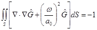
From the Gauss’ Divergence Theorem we have:
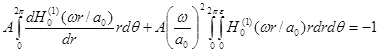
As ![]() ,
,
![]() ,
,
![]() .
.
Therefore,
![]() ,
,
This is the two-dimensional Green’s function in a stationary medium in Cartesian coordinates in frequency domain. It has the logarithmic singularity at the origin. The 2D Green’s function in cylindrical coordinates is referred to Eq.(7.3.18) in Morse&Ingard1968.
In the limit of incompressible medium, ![]() . The
non-homogeneous equation is:
. The
non-homogeneous equation is:
![]() .
.
One
may find its Green’s function by performing the limiting analysis of (136) as ![]() . But the correct way is to use the similar
procedure from (133) to (136), which leads to this Green’s function in
two-dimensional stationary incompressible medium:
. But the correct way is to use the similar
procedure from (133) to (136), which leads to this Green’s function in
two-dimensional stationary incompressible medium:
![]() .
()
.
()
2D Green’s Function in Subsonic Mean Flow
(Cf.Howe1998, p.38)
When
![]() and
and
![]() , we can use the Prandtl-Glauert transformation
(83) to transform Eq.(131) into:
, we can use the Prandtl-Glauert transformation
(83) to transform Eq.(131) into:
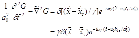
According to (136), the solution to (137) in two dimensions is:
In the original coordinates it is:
Eq.(138) is the Green’s function in a subsonic mean flow for Eq.(131).
Green’s Function in Three Dimensional Open Space with Mean Flow
Eq.(69) is the non-homogeneous equation for the Green's function in a three-dimensional flow:
![]()
Applying the Prandtl-Glauert transformation (83) in Eq.(69), one obtains
![]() . (139)
. (139)
The Green's function in a stationary medium is provided by Eq.(66). Therefore, the solution to Eq.(139) in three dimensions is
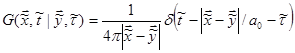 .
.
Reverting it to the original coordinates, one obtains the Green's function for uniform mean flows:
![]() [GE11] .
(140)
[GE11] .
(140)
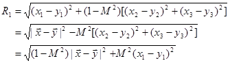
![]()
Note
![]() : amplification of mean flow.
: amplification of mean flow.
C.f. Michalke&Michel1979, Eq.(3.2), Ikeda et al 2016, Eq.(8), Najafi-Yazdi et al 2011, Eq. (2.24), Howe1998, Eq.(1.7.17) for frequency domain.