Sound
Propagation in Ducts
Hongbin Ju
www.aeroacoustics.info
hju@math.fsu.edu
In this section we discuss sound
propagation in ducts. This is a typical case of acoustic waves in a confined
environment. In the wall bounded directions, acoustic waves bounce back and forth
to form standing wave patterns. In the axial direction acoustic waves propagate
freely. We will show how to solve acoustic equations for these boundary conditions.
The theory developed is very useful in applications such as the prediction and
control of aircraft engine noise.
Sound Propagation in Rectangular Duct
Assume a uniform
subsonic mean flow
in a rectangular duct with width d
and height h. The mean flow density is
![]() , pressure
, pressure ![]() , and velocity
, and velocity ![]() in +x-axis direction.
in +x-axis direction.
The scales used are: length L, velocity: sound speed ![]() , time
, time ![]() , density: ambient density
, density: ambient density ![]() , pressure:
, pressure: ![]() , impedance:
, impedance: ![]() . The linear Euler
equations for the fluctuation quantities are:
. The linear Euler
equations for the fluctuation quantities are:
![]() ,
(0-1)
,
(0-1)
![]() ,
(0-2)
,
(0-2)
![]() ,
(0-3)
,
(0-3)
![]() . (0-4)
. (0-4)
Variables
without bars are perturbation quantities. Isentropic process is assumed;
therefore density
can be calculated from pressure: ![]() ,
, ![]() .
.
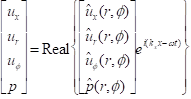
We use the trial
solution and the
method of separation of variables to
solve the equations. In the y- and z- directions there are wall boundaries.
In the x- direction the duct extends
to infinity. Assume the next form of solutions:
 (1)
(1)
Substituting (1) into the linear Euler
equations, one obtains the following acoustic equations:
![]() ,
, ![]() ,
, ![]() , (3)
, (3)
when
![]() . The linear Euler
equations with the isentropic process have two normal modes: acoustic mode (
. The linear Euler
equations with the isentropic process have two normal modes: acoustic mode (![]() , phase speed not equal to flow velocity), and vortical mode (
, phase speed not equal to flow velocity), and vortical mode (![]() , phase speed equal to flow velocity). We are only interested in the acoustic modes; therefore
, phase speed equal to flow velocity). We are only interested in the acoustic modes; therefore ![]() and the acoustic
equations in Eqs.(2&3) are chosen according to cht1.doc.
and the acoustic
equations in Eqs.(2&3) are chosen according to cht1.doc.
Rigid Wall Duct with Mean Flow
If the duct walls are rigid, the boundary conditions are
![]() , at
, at ![]() and
and ![]() ; (4)
; (4)
![]() , at
, at ![]() and
and ![]() . (5)
. (5)
In the flow direction the wave
amplitude must remain finite as ![]() .
.
We try the separation of
variable:
![]() .
.
Substituting it into (2) leads
to:
![]() .
.
The first term on the left
depends on y only. The second term
depends on z only. ![]() is constant with respect
to y and z. Therefore the following equations must be true:
is constant with respect
to y and z. Therefore the following equations must be true:
![]() ,
, ![]() ,
, ![]() .
(5-1)
.
(5-1)
![]() and
and ![]() are constants. One can
use the trial solution method to solve the two ODEs in (5-1). The general
solution is:
are constants. One can
use the trial solution method to solve the two ODEs in (5-1). The general
solution is:
![]() . (6)
. (6)
To satisfy boundary conditions
(4) and (5), we must have
![]() ,
, ![]() ;
(7)
;
(7)
![]() ,
, ![]() .
(8)
.
(8)
m
and n can be any integers. Usually we use
non-negative integers: ![]() ,
, ![]() . Due to the wall confinements, wave numbers
. Due to the wall confinements, wave numbers ![]() and
and ![]() can no longer be any
real numbers. They must be multiples of
can no longer be any
real numbers. They must be multiples of ![]() and
and ![]() respectively. For this reason,
respectively. For this reason, ![]() and
and ![]() are called
eigenvalues. With (7) and (8), solution (6) is:
are called
eigenvalues. With (7) and (8), solution (6) is:
It represents the standing
waves in both the y and z directions. (Compared with the
plane wave solutions discussed in cht1.doc.) Amplitude ![]() is to be determined
by acoustic sources in the duct and the boundary conditions in the x direction.
is to be determined
by acoustic sources in the duct and the boundary conditions in the x direction. ![]() and
and ![]() are called
the eigenfunctions. Each pair of (m,n) represents one acoustic mode with the
solution (9) to Eq.(2). It is called a normal
mode of the acoustic field.
are called
the eigenfunctions. Each pair of (m,n) represents one acoustic mode with the
solution (9) to Eq.(2). It is called a normal
mode of the acoustic field.
According
to Eq.(5-1), (7), and (8), eigenvalue
![]() is
determined by the duct geometry:
is
determined by the duct geometry:
![]() . (10)
. (10)
Eq.(2)
implies only ![]() matters; therefore
only the positive square root is chosen.
matters; therefore
only the positive square root is chosen. ![]() is real and positive for the rigid wall duct. For
each eigenvalue
is real and positive for the rigid wall duct. For
each eigenvalue ![]() , there are two solutions of
, there are two solutions of ![]() from
Eq.(2):
from
Eq.(2):
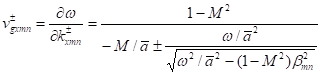
They represent waves propagating
in opposite directions in x. The
direction of a wave is determined by group velocity. If ![]() ,
, ![]() is real and the mode is cut-on. Taking the derivative with
respect to
is real and the mode is cut-on. Taking the derivative with
respect to ![]() in Eq.(11), we obtain
the group velocity
in Eq.(11), we obtain
the group velocity
 [hj1] .
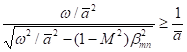
Since
![]() , the wave with
, the wave with ![]() propagates in the -x direction. Noting
propagates in the -x direction. Noting
 ,
,
![]() ,
,
the wave with ![]() propagates in the +x direction.
propagates in the +x direction.
If ![]() , we have
, we have
![]()
![]()
![]()
![]() ,
,
![]() , (11-0)
, (11-0)
![]() .
.
i, not –i, is chosen for the square root so ![]() has positive imaginary
part and
has positive imaginary
part and ![]() has negative imaginary
part. The imaginary part of
has negative imaginary
part. The imaginary part of ![]() provides exponential
attenuation factor
provides exponential
attenuation factor ![]() in
in ![]() in Eq.(1), with which the
wave amplitude remains finite as
in Eq.(1), with which the
wave amplitude remains finite as ![]() .
. ![]() represents an evanescent or
cut-off mode.
represents an evanescent or
cut-off mode.
The mode becomes cut-on if the frequency increases so that:
![]() . (11-1)
. (11-1)
![]() is the cut-off frequency of mode (m,n). The cutoff ratio is defined as
(Hubbard1995, p.159):
is the cut-off frequency of mode (m,n). The cutoff ratio is defined as
(Hubbard1995, p.159):
![]() . (11-2)
. (11-2)
![]() represents
propagating, or cut-on, modes. The
number of cut-on modes is limited at any frequency. A mean flow makes a mode easier
to cut on. A plane wave is always cut-on:
represents
propagating, or cut-on, modes. The
number of cut-on modes is limited at any frequency. A mean flow makes a mode easier
to cut on. A plane wave is always cut-on: ![]() ,
, ![]() ,
, ![]() ,
, ![]() .
.
It is noted that the eigenvalues
and eigenfunctions in the y or z direction are solely determined by the
boundary conditions. They are independent of wave propagating directions. This is
not true when there is mean flow and the walls are not rigid, as will be discussed
later.
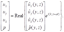
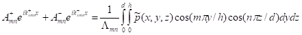
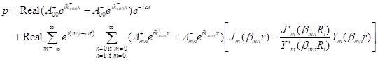
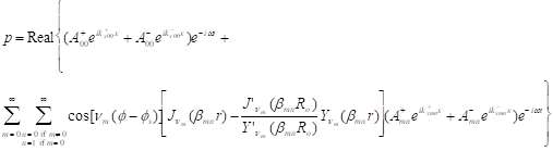
Substituting (9) into (1) and summing
up all possible modes, we obtain the general solution of acoustic pressure:
Acoustic velocities can be calculated
from Eq.(3). This solution represents a general sound field in a rectangular
rigid-wall duct. Any specific pressure field can be expanded to the sum of normal
modes of the rectangular duct. The amplitude of each mode ![]() is
determined by the sound sources and the boundary conditions in the x direction. Mode (m,n) is present in the
sound field, or excited by the source, if
is
determined by the sound sources and the boundary conditions in the x direction. Mode (m,n) is present in the
sound field, or excited by the source, if ![]() .
.
Given the total pressure field ![]() , how to calculate amplitude
, how to calculate amplitude ![]() of each individual
mode? It is noted that eigenfunctions
of each individual
mode? It is noted that eigenfunctions ![]() are
orthogonal:
are
orthogonal:
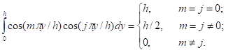
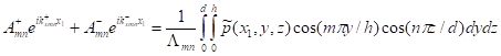
The
same is true for ![]() . One can calculate
the jth component of pressure using
the orthogonality. Applying (12-1) on
(12) and integrate the equation on the duct section at x, we have:
. One can calculate
the jth component of pressure using
the orthogonality. Applying (12-1) on
(12) and integrate the equation on the duct section at x, we have:
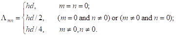
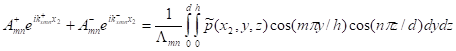
Modes (m,n) are obtained by filtering out all other modes through the integration.
Depending on locations of sound sources and duct terminations, one can further
separate amplitudes ![]() and
and ![]() . For
example, if sound sources are at the left side of the section and at the right
hand side the duct extends to infinity (no reflection from this end), then
. For
example, if sound sources are at the left side of the section and at the right
hand side the duct extends to infinity (no reflection from this end), then
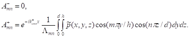 (12-3)
If waves propagate towards this
section from both sides, the integration (12-2) at two axial locations ![]() and
and ![]() are needed and
are needed and ![]() and
and ![]() can be solved from the
linear equations:
can be solved from the
linear equations:
 .
.
For a rigid-wall duct, ![]() is real so
is real so ![]() can be calculated
by (11) for cut-on modes
and (11-0) for cut-off modes. In many practical problems such as in lined
ducts,
can be calculated
by (11) for cut-on modes
and (11-0) for cut-off modes. In many practical problems such as in lined
ducts, ![]() is complex. Then branch
cuts must be inserted for
is complex. Then branch
cuts must be inserted for ![]() and
and ![]() in (11-0) to make them single-valued. The branch cuts
must be chosen so that the imaginary part of
in (11-0) to make them single-valued. The branch cuts
must be chosen so that the imaginary part of
![]()
![]() is not negative so the magnitude of the wave
is finite as
is not negative so the magnitude of the wave
is finite as ![]() .
.
We choose the branch cuts as
shown in Fig.1, with which the phase range of ![]()
![]() is
is ![]() . The
phase range for
. The
phase range for ![]() in (11-0) is
in (11-0) is ![]() so the amplitude of
the right-propagating wave with factor
so the amplitude of
the right-propagating wave with factor ![]() remains finite as
remains finite as ![]() . The phase range for
. The phase range for ![]() is
is ![]() and amplitude of the left-propagating
wave remains finite as
and amplitude of the left-propagating
wave remains finite as ![]() .
.
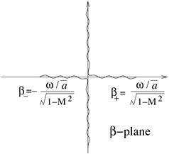
Fig.1, Branch cuts for ![]() and
and ![]() on the
on the ![]() -plane[hj2] .
-plane[hj2] .
Sometimes we need to calculate
eigenvalue ![]() from wave number
from wave number ![]() :
:
![]() ,
(13-1)
,
(13-1)
![]() ,
, ![]() .
.
Branch cuts for ![]() and
and ![]() are chosen as in Fig.2. The phase range of
are chosen as in Fig.2. The phase range of ![]() is
is ![]() . The
phase range of
. The
phase range of ![]() is
is ![]() so the real part of
so the real part of ![]() is always positive.
is always positive.
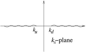
Fig.2, Branch cuts for ![]() and
and ![]() on the
on the ![]() -plane.
-plane.
Soft Wall Duct without Mean Flow
To simplify the problem, we assume no mean flow in the duct and the same impedance in the opposite walls. The boundary conditions are:
![]() at
at ![]() ,
, ![]() at
at ![]() ; (13)
; (13)
![]() at
at ![]() ,
, ![]() at
at ![]() . (14)
. (14)
![]() and
and ![]() are admittance of the
soft walls.
are admittance of the
soft walls.
We can still use the trial
solution Eq.(6). To facilitate the derivation, we rewrite Eq.(6) as:
![]() (15)
(15)
by defining ![]() ,
, ![]() ,
, ![]() , and
, and ![]() .
.
To satisfy boundary conditions
(13) in the y direction, we must have
![]() ; (16)
; (16)
![]() .
(17)
.
(17)
From which we have,
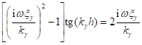 . (18)
Eigenvalue ![]() can be solved from
this equation using the grid search/Newton iteration method.
can be solved from
this equation using the grid search/Newton iteration method.
Another way to solve equations (16) and (17) is to note:
![]() .
(19)
.
(19)
One
possible solution is ![]() , then:
, then:
![]() ,
,
![]() ,
(20)
,
(20)
which corresponds to the even symmetric solution in Morse&Ingard1968, p.504.
The
other possible solution to Eq.(19) is ![]() , i.e.,
, i.e.,
![]() ,
,
![]() .
(21)
.
(21)
which
corresponds to the odd symmetric solution in Morse&Ingard1968, p.504.
Similarly ![]() can be solved.
Eigenvalue
can be solved.
Eigenvalue ![]() or
or ![]() is the same for the
wave propagating in +x or -x direction. However, eigenfunctions
is the same for the
wave propagating in +x or -x direction. However, eigenfunctions ![]() or
or ![]() are no longer
orthogonal as in the hard wall case.
are no longer
orthogonal as in the hard wall case.
If
there is a mean flow in the soft wall duct, eigenvalues
![]() and
and ![]() are no longer
independent of the wave propagation direction in x. They are different for the different propagation directions.
This will be further discussed in the following section about the soft wall
circular duct.
are no longer
independent of the wave propagation direction in x. They are different for the different propagation directions.
This will be further discussed in the following section about the soft wall
circular duct.
Sound Propagation in Circular Duct
Scales used here are: length:
duct diameter D, velocity: sound
speed ![]() , time:
, time: ![]() , density: density
, density: density ![]() , pressure:
, pressure: ![]() , impedance:
, impedance: ![]() .
.
The mean flow: ![]() and
and ![]() are constant; mean
velocity
are constant; mean
velocity ![]() is in +x-axis direction and constant.
is in +x-axis direction and constant.
The Euler equations for the
fluctuation quantities are:
![]() , (21-1)
, (21-1)
![]() , (21-2)
, (21-2)
![]() , (21-3)
, (21-3)
![]() .
(21-4)
.
(21-4)
(Density can be calculated
directly from pressure: ![]() ,
, ![]() .)
.)
In the radial direction there is
a wall boundary and in the circumferential direction there is a periodic
boundary. In the x direction the duct
extends to infinity. We assume the form of solutions:
 . (22)
Substituting it into the Euler
equations, we have:
![]() , (23)
, (23)
![]() ,
, ![]() ,
, ![]() . (24)
. (24)
where
![]() .
. ![]() is the dispersion
relationship for circular/annular ducts.
is the dispersion
relationship for circular/annular ducts.
To
solve ![]() from Eq.(23), assume
the separation of variables:
from Eq.(23), assume
the separation of variables:
![]() .
(25)
.
(25)
Substitute it into Eq.(23),
![]() .
.
The left hand side of the equation
depends on r only. The right hand side
is only a function of ![]() . Then they must be equal to the same constant:
. Then they must be equal to the same constant:
![]() ,
(26)
,
(26)
![]() . (27)
. (27)
The general solution to Eq.(26) is:
![]() .
(28)
.
(28)
A, B
and ![]() are to be determined
by two boundary conditions in the
are to be determined
by two boundary conditions in the ![]() direction.
direction.
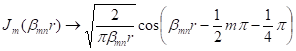
Solutions
to Eq.(27) are Bessel functions. It is either Bessel function of the first kind
![]() representing
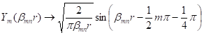
standing waves in the radial direction in a circular duct, or the second kind
representing
standing waves in the radial direction in a circular duct, or the second kind ![]() for standing waves in annular ducts, or Hankel
functions
for standing waves in annular ducts, or Hankel
functions ![]() and
and ![]() (the third kind
of Bessel functions) representing propagating waves (outward/inward, no ducts).
The general solution in the duct is:
(the third kind
of Bessel functions) representing propagating waves (outward/inward, no ducts).
The general solution in the duct is:
![]() .
(29)
.
(29)
![]() ,
, ![]() are
respectively the
are
respectively the ![]() th order first and second kinds of Bessel functions. They are
two independent solutions to Bessel equation (27). C, D and
th order first and second kinds of Bessel functions. They are
two independent solutions to Bessel equation (27). C, D and ![]() are determined by two
boundary conditions in the radial
direction.
are determined by two
boundary conditions in the radial
direction.
For
a circular duct, the periodic boundary condition
applies in ![]() direction. The general
solution to Eq.(26) is:
direction. The general
solution to Eq.(26) is:
![]() ,
(30)
,
(30)
where ![]() is an integer. In the
radial direction, the boundary condition at
is an integer. In the
radial direction, the boundary condition at ![]() is that
is that ![]() must be finite.
must be finite. ![]() is eliminated since it
is infinitive at
is eliminated since it
is infinitive at ![]() . Therefore the general solution of
. Therefore the general solution of ![]() is
is
![]() .
(31)
.
(31)
The general solution of ![]() for a circular duct
is:
for a circular duct
is:
![]() .
(32)
.
(32)
![]() is to be determined by
the boundary condition at
is to be determined by
the boundary condition at ![]() . (
. (![]() is the radius of the
duct.) All other
variables can be computed from
is the radius of the
duct.) All other
variables can be computed from ![]() by Eq.(24).
by Eq.(24).
As |m| increases, ![]() is small for small r and large for large r. Sound energy concentrates near the
cylindrical duct wall for high |m| mode.
is small for small r and large for large r. Sound energy concentrates near the
cylindrical duct wall for high |m| mode.
Rigid Wall Circular Duct
For
a rigid wall duct, the boundary condition at
![]() is
is
![]() .
(33)
.
(33)
To satisfy (33), one has the
eigenvalue:
![]() , (34)
, (34)
where ![]() is the nth root of
is the nth root of ![]() . (See Appendix for how to find
. (See Appendix for how to find ![]() .) Since
.) Since ![]() , eigenvalues are the same for
, eigenvalues are the same for ![]() :
: ![]() . And eigenfunctions satisfy:
. And eigenfunctions satisfy: ![]() .
.
The
time domain solution of p is:
![]() . (35)
. (35)
![]() and
and ![]() are the same for both directions in x.
are the same for both directions in x. ![]() is orthogonal. (This is not true when there is
mean flow and the duct wall is not rigid.) Wave number
is orthogonal. (This is not true when there is
mean flow and the duct wall is not rigid.) Wave number ![]() can be computed from
Eq.(11) and the cut-on frequency from Eq.(11-1). For larger azimuthal mode
(larger |m|),
can be computed from
Eq.(11) and the cut-on frequency from Eq.(11-1). For larger azimuthal mode
(larger |m|), ![]() is larger, so is the
cut-on frequency. Therefore there is less number of cut-on radial modes for
larger |m|.
is larger, so is the
cut-on frequency. Therefore there is less number of cut-on radial modes for
larger |m|.
Soft Wall Circular Duct
Assume a plug flow in the duct. The tangential discontinuity at the disturbed surface leads to the continuity of displacement at the wall (cht21.doc) and the Myer’s impedance boundary condition (cht24.doc):
![]() at
at ![]() . (35-1)
. (35-1)
Plugging
![]() in Eq.(32) and
in Eq.(32) and ![]() in Eq.(24) into
the Myer’s boundary condition, we have:
in Eq.(24) into
the Myer’s boundary condition, we have:
![]() . (35-2)
. (35-2)
It
is not trivial to solve eigenvalue ![]() from this equation.
The grid search/Newton’s iteration method can be used. With mean flow,
from this equation.
The grid search/Newton’s iteration method can be used. With mean flow, ![]() is coupled with
is coupled with ![]() . Therefore, it is no longer independent of the wave
propagation direction as in the no flow soft wall case or as in the solid wall
with mean flow case.
. Therefore, it is no longer independent of the wave
propagation direction as in the no flow soft wall case or as in the solid wall
with mean flow case. ![]() is different for waves
propagating in +x and –x direction for soft wall duct with mean
flow.
is different for waves
propagating in +x and –x direction for soft wall duct with mean
flow.
Sound Propagation
in Annular Duct
An annular duct has an inner circular wall
with radius ![]() and an outer circular
wall with radius
and an outer circular
wall with radius ![]() . The equations are (21-1)~(21-4), with scales: length: outer
duct diameter
. The equations are (21-1)~(21-4), with scales: length: outer
duct diameter ![]() ,
velocity: sound speed
,
velocity: sound speed ![]() , time:
, time: ![]() , density: density
, density: density ![]() , pressure:
, pressure: ![]() , impedance:
, impedance: ![]() . And the solution form is (22).
. And the solution form is (22).
The
analysis of the periodic
boundary condition and the
general solution (30) for the circular duct still apply in the annular duct. In the radial
direction, ![]() is not in the physical
domain as in the circular duct. Therefore
is not in the physical
domain as in the circular duct. Therefore ![]() in Eq.(29) should be
kept in the general solution:
in Eq.(29) should be
kept in the general solution:
![]() . (36)
. (36)
C, D and ![]() are to be determined by two
boundary conditions at
are to be determined by two
boundary conditions at ![]() and
and ![]() . With
. With ![]() , sound
energy doesn’t concentrate near the outer duct wall for high mode m as in a cylindrical duct.
, sound
energy doesn’t concentrate near the outer duct wall for high mode m as in a cylindrical duct.
Rigid Wall Annular Duct
For a rigid wall annular duct, the boundary conditions are
![]() , at
, at ![]() and
and ![]() . (37)
. (37)
First of all, one should check if
![]() is the eigenvalue. Since
is the eigenvalue. Since
![]() ,
, ![]() must be zero and
must be zero and ![]() . Since
. Since ![]() for
for ![]() ,
, ![]() for
for ![]() , the only nontrivial solution to Eq.(36) is:
, the only nontrivial solution to Eq.(36) is:
![]() ,
, ![]() . (38)
. (38)
This represents a plane wave. The
plane wave in a circular or annular duct only propagates in the axial direction.
For all the cases other than ![]() and
and ![]() , we have
, we have ![]() . From boundary condition (37), the dispersion relation is
obtained from (36):
. From boundary condition (37), the dispersion relation is
obtained from (36):
![]() . (39)
. (39)
The
prime denotes the derivative with respect to the whole argument. It is not
trivial to solve eigenvalue
![]() from Eq.(39). When the
gap of annular duct
from Eq.(39). When the
gap of annular duct ![]() is much smaller than
is much smaller than ![]() , we can obtain an approximate solution of
, we can obtain an approximate solution of ![]() . We begin with the Bessel equation (27). By replacing
. We begin with the Bessel equation (27). By replacing ![]() by the medium radius
by the medium radius ![]() , the Bessel equation becomes a second order ODE with
constant coefficients:
, the Bessel equation becomes a second order ODE with
constant coefficients:
![]() . (39-1)
. (39-1)
Its general solution is:
![]() ,
,  .
.
![]() and
and ![]() are both real, or a
conjugate pair.
are both real, or a
conjugate pair.
To satisfy boundary conditions (37),
![]() ,
,
i.e.,
Therefore the eigenvalue for an annular duct with small gap is
 , n=0, 1, 2, ..... (40)
According to Eq.(11-2), for a cut-on mode in a narrow annular duct, n must be zero. Therefore
![]() [hj4] .
[hj4] .
For large m,
![]() .
.
As ![]() , does the narrow annular approaches a rectangular duct?
Compare Eq.(40) with Eq.(10). The radial wavenumber in the annular duct
, does the narrow annular approaches a rectangular duct?
Compare Eq.(40) with Eq.(10). The radial wavenumber in the annular duct ![]() approaches the height
mode,
approaches the height
mode, ![]() . The spinning mode wavenumber
. The spinning mode wavenumber ![]() approaches the depth
mode. However, there is an extra wavenumber
approaches the depth
mode. However, there is an extra wavenumber ![]() in the annular duct. It
comes from term
in the annular duct. It
comes from term ![]() in Eq.(39-1), which
does not exist in the rectangular duct Eq.(5-1). If m is kept constant as
in Eq.(39-1), which
does not exist in the rectangular duct Eq.(5-1). If m is kept constant as ![]() , then
, then 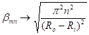 . It is equivalent to regular duct with uniform mode shape in
the depth direction. On the other hand, if
. It is equivalent to regular duct with uniform mode shape in
the depth direction. On the other hand, if ![]() remains constant as
remains constant as ![]() , then
, then ![]() and
and 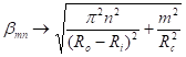 . The annular duct approaches a rectangular duct. For the
mode shape, as
. The annular duct approaches a rectangular duct. For the
mode shape, as ![]() ,
, ![]() , Eq.(36)
, Eq.(36)
 ,
,
 .
.
Compare it with Eq.(12), it approaches rectangular duct height mode shape.
Another asymptotic formula for the eigenvalues based on the WKB method was developed by Envia. (Envia1998, Eq.9)
One may solve Eq.(39) numerically using the Newton iteration method. Define function:
![]() [HB5] .
[HB5] .
For
initial eigenvalue ![]() , the improved eigenvalue is
, the improved eigenvalue is
![]() ,
, ![]()
![]() . This process is repeated until
. This process is repeated until ![]() is small. A successful
Newton method depends on a good initial eigenvalue
is small. A successful
Newton method depends on a good initial eigenvalue ![]() . The next figure shows a typical
. The next figure shows a typical ![]() . Separate
. Separate ![]() -axis into intervals, ...,
-axis into intervals, ..., ![]() ,
,![]() ,.... If
,.... If ![]() ,
, ![]() is a good choice of
is a good choice of ![]() . A FORTRAN90 code, modenumber_annularduct.f, using this
method to compute eigenvalues in a solid wall annular duct is attached.
. A FORTRAN90 code, modenumber_annularduct.f, using this
method to compute eigenvalues in a solid wall annular duct is attached.
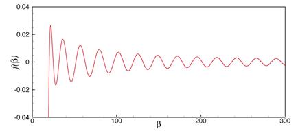
m=18, ![]() ,
, ![]() .
.
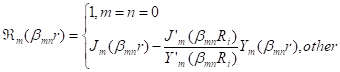
One
can show that ![]() . Therefore eigenvalues for m are also the eigenvalues for –m:
. Therefore eigenvalues for m are also the eigenvalues for –m:
![]() . Eigenfunction for (-m,n)
is the same as for (m,n).
. Eigenfunction for (-m,n)
is the same as for (m,n).
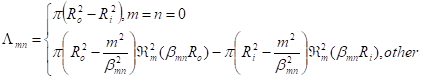
A general solution of ![]() is then:
is then:
![]() , m=n=0;
, m=n=0;
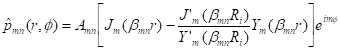 , other. (40-1)
Velocities are computed by
Eq.(24). Wave number ![]() can be computed from
Eq.(11) & (11-0).
can be computed from
Eq.(11) & (11-0).
The
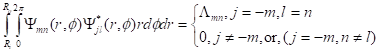
time domain solution of p is:
Orthogonality:
According to Abramowitz&Stegun1964, Eq.(11.4.2), p.485,
![]()
Cut-on ratio
For annular ducts the cut-on ratio in
Eq.(11-2) can be rewritten as
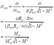 ,
,
![]() ,
, ![]() .
.
![]() is the phase speed in
the circumferential direction.
is the phase speed in
the circumferential direction. ![]() is called the cut-off
Mach number. It is roughly the ratio of radial wavenumber and the
circumferential wavenumber. For narrow ducts,
is called the cut-off
Mach number. It is roughly the ratio of radial wavenumber and the
circumferential wavenumber. For narrow ducts, ![]() . This is true for any ducts. For narrow ducts and large m,
. This is true for any ducts. For narrow ducts and large m, ![]() . For arbitrary annular ducts,
. For arbitrary annular ducts, ![]() depends on the hub/tip
ratio and m:
depends on the hub/tip
ratio and m:
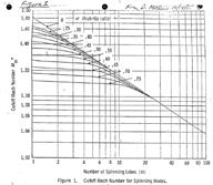
If for large m in narrow ducts without axial mean flow, the phase speed of the
mode in the circumferential direction must be supersonic to be cut-on.
Sound
Propagation C-Duct
In
the outlet of jet engines, the annular duct is often separated by
installations, as illustrated by Fig.3. The duct has a C-shape. It is here
called C-duct. The C-duct has an
inner duct with radius ![]() and an outer duct with
radius
and an outer duct with
radius![]() . The separation plates are at
. The separation plates are at ![]() and
and ![]() .
.
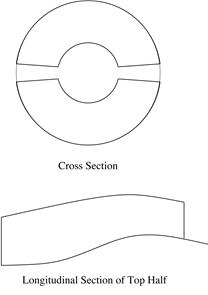
Fig.3, C-duct.
The first major difference of
C-duct from the annular duct is the periodic boundary condition is no
longer applicable in the ![]() direction. Because of
the presence of the bifurcations, spinning duct modes are not possible.
Reflections at the bifurcations lead to the formation of a standing wave
pattern in the cross-section of the duct. Similar to the argument for Eq.(9) in
rectangular duct, the general solution of
direction. Because of
the presence of the bifurcations, spinning duct modes are not possible.
Reflections at the bifurcations lead to the formation of a standing wave
pattern in the cross-section of the duct. Similar to the argument for Eq.(9) in
rectangular duct, the general solution of ![]() is:
is:
![]() , (42)
, (42)
where
![]() ,
, ![]() . (43)
. (43)
m is any nonnegative integer. ![]() may not be an integer
as in the circular or annular duct unless when
may not be an integer
as in the circular or annular duct unless when ![]() . (When
. (When ![]() , the solution in a C duct is the same as that in an annular
duct.)
, the solution in a C duct is the same as that in an annular
duct.)
In the radial direction the
general solution is:
![]() . (44)
. (44)
The second major difference of
the C-duct from annular duct is the Bessel functions here may have non-integer
orders.
Rigid Wall C-Duct
For the rigid wall C-duct, the boundary conditions in radial direction are
![]() , at
, at ![]() and
and ![]() . (45)
. (45)
The similar argument as for
Eq.(38) leads to the plane wave solution:
![]() ,
, ![]() .
(46)
.
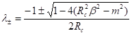
(46)
If ![]() , the next dispersion relation can be derived from (44) and
(45):
, the next dispersion relation can be derived from (44) and
(45):
![]() .
(47)
.
(47)
Eigenvalue ![]() is to be determined by
this equation. The difficulty involved here is the Bessel functions with
non-integer order.
is to be determined by
this equation. The difficulty involved here is the Bessel functions with
non-integer order.
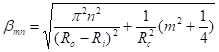
From the similar procedures for
Eq.(40), when the gap of annular duct, ![]() , is small, the eigenvalue is approximated by:
, is small, the eigenvalue is approximated by:
![]() , n=0,1,2,..... (48)
, n=0,1,2,..... (48)
If the gap of the annular duct is not small, we can use (48) as an initial value in a Newton iteration method. The final results need to be reorganized.
The
time domain solution of p is:
 . (49)
With solution of ![]() , all
other variables can be computed from Eq.(24).
, all
other variables can be computed from Eq.(24).
Sound Propagation in Circular Duct with Nonuniform Mean Flow (Boundary Layer)
Scales used will be: length: duct
radius R, velocity: sound speed ![]() , density: ambient density
, density: ambient density ![]() , pressure:
, pressure: ![]() , impedance:
, impedance: ![]() .
.
The mean flow: ![]() and
and ![]() (
(![]() ) are constant; Shear mean velocity
) are constant; Shear mean velocity ![]() is in +x-axis direction.
is in +x-axis direction.
Assume the next form of
solutions:
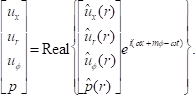 (50)
(50)
(Density can be computed directly
from pressure: ![]() .)
.)
From Euler equations, one can
obtain the next equations for shear flow:
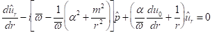 ,
(51)
,
(51)
![]() ,
(52)
,
(52)
where
![]() . For a wall with impedance Z, the boundary condition is
. For a wall with impedance Z, the boundary condition is
![]() , at
, at ![]() .
(53)
.
(53)
Equations (51) and (52) and
boundary condition (53) form an eigenvalue problem. Only some special values of
![]() can satisfy these
equations. These
can satisfy these
equations. These ![]() are eigenvalues, and the respective
functions
are eigenvalues, and the respective
functions ![]() and
and ![]() are eigenfunctions.
are eigenfunctions.
An important property of
eigenvalues of Eqs.(51)&(52) is given here. Suppose ![]() ,
, ![]() ,
, ![]() are a set of
eigenvalue and eigenfunctions of this problem, then
are a set of
eigenvalue and eigenfunctions of this problem, then ![]() ,
, ![]() ,
, ![]() form a set of
eigenvalue and eigenfunctions for Eqs.(51)&(52) satisfying the next B.C.:
form a set of
eigenvalue and eigenfunctions for Eqs.(51)&(52) satisfying the next B.C.:
![]() , at
, at ![]() .
(54)
.
(54)
Here
superscript * represents conjugate. Under some circumstances B.C.(53) is exactly the same as
B.C.(54), such as for hard wall, ![]() , or the impedance with only resistance,
, or the impedance with only resistance, ![]() . Then
. Then ![]() ,
, ![]() ,
, ![]() are also the set of
eigenvalue and eigenfunctions for the original problem [Eqs.(51)&(52) with
B.C.(53)].
are also the set of
eigenvalue and eigenfunctions for the original problem [Eqs.(51)&(52) with
B.C.(53)].
Newton
iteration method
can be used to solve the eigenvalues and eigenfunctions. For an initial guess
of the eigenvalue ![]() , integrate Eqs.(51)&(52) numerically from the outside of
the boundary layer to
, integrate Eqs.(51)&(52) numerically from the outside of
the boundary layer to ![]() to get
to get ![]() and
and ![]() at
at ![]() .
. ![]() and
and ![]() are functions of
are functions of ![]() :
: ![]() ,
, ![]() , which may not satisfy B.C. (53) at
, which may not satisfy B.C. (53) at ![]() . Similarly we can have another solution
. Similarly we can have another solution ![]() and
and ![]() for initial eigenvalue
for initial eigenvalue
![]() near
near ![]() . Suppose
the exact eigenvalue is
. Suppose
the exact eigenvalue is ![]() , i.e.,
, i.e.,
![]() .
.
To the first order of Taylor
expansion, we have:
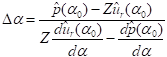 .
.
If we use ![]() ,
, ![]() , we can get
, we can get ![]() to have a better
approximation to the accurate eigenvalue. The process can be repeated until
certain accuracy is achieved. This is the Newton’s iteration method.
to have a better
approximation to the accurate eigenvalue. The process can be repeated until
certain accuracy is achieved. This is the Newton’s iteration method.
Choosing appropriate initial
value ![]() is critical for a
successful Newton’s iteration method. Eigenvalues of plug flow without boundary
layer, Eq.(34) and Eq.(11), are good choice of the initial eigenvalues. In most
of the time these choices work well. But in some cases Newton’s method fail
when using these initial eigenvalues.
is critical for a
successful Newton’s iteration method. Eigenvalues of plug flow without boundary
layer, Eq.(34) and Eq.(11), are good choice of the initial eigenvalues. In most
of the time these choices work well. But in some cases Newton’s method fail
when using these initial eigenvalues.
Another way for choosing initial
eigenvalues is the grid search.
Compute function:
![]() (55)
(55)
for a matrix in ![]() -plane, draw the contours of real(f)=0 and imag(f)=0 in the
-plane, draw the contours of real(f)=0 and imag(f)=0 in the
![]() -plane using a commercial software. The intersection points
in the
-plane using a commercial software. The intersection points
in the ![]() -plane should be the solution of the eigenvalues. Read in
these data and use them as the initial eigenvalues in the Newton iteration.
-plane should be the solution of the eigenvalues. Read in
these data and use them as the initial eigenvalues in the Newton iteration.
As an example, let's find eigenvalues for mean flow with turbulent boundary layer in a circular rigid wall duct with radius: 62.33”. The velocity profile of the turbulent boundary layer is shown in Fig.4. Mach number: 0.452, boundary layer thickness: 1”,
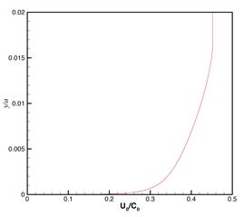
Fig.4, Velocity profile of
turbulent boundary layer, Mach number: 0.452, boundary layer thickness:
1”.
The grid search method is used to
get the initial guess of eigenvalues. Since the wall is rigid, both ![]() and
and ![]() are the eigenvalues
according to the property discussed above. Therefore in Fig.5 only the up half
of the
are the eigenvalues
according to the property discussed above. Therefore in Fig.5 only the up half
of the ![]() -plane is needed. Read in the data of the intersection points
of solid and dashed lines as the initial values in the Newton’s method.
-plane is needed. Read in the data of the intersection points
of solid and dashed lines as the initial values in the Newton’s method.
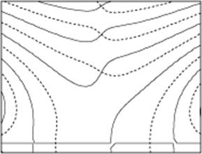
Fig.5, Contours of real(f)=0 (solid lines) and imag(f)=0 (dashed lines) in the ![]() -plane
-plane
The next figures show the
results. Fig.6 shows the eigenvalues when frequency is just above the cut-on
frequency. Fig.7 is for frequency is well above the cut-on frequency. Fig.8 is
for frequency well below the cut-on frequency. In most of the cases, the effect
of shear flow is to move real parts of plug flow eigenvalues to right while the
imaginary parts keep nearly the same. This change is very small. Using plug
flow eigenvalues as initial values in Newton method works well. The only exception is when the
frequency is just above the cut-on frequency (Fig6). There are two cut-on modes
in the plug flow. The boundary layer makes these propagating modes into cut-off
modes. This explains why a cut-on mode wave was damped in experiments. In this
case the plug flow eigenvalues as the initial value fails.
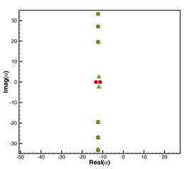
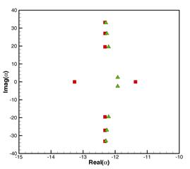
Fig.6,
Eigenvalues at 741Hz for plug flow (square) and shear flow with turbulent
boundary layer (triangle). Mach number: 0.452, boundary layer thickness: 1”,
duct radius: 62.33”, azimuthal mode number m=22,
cut-on frequency for the 1st radial mode of the plug flow: 740.6Hz.
[Real(![]() ) in the right figure is rescaled to show the difference.]
) in the right figure is rescaled to show the difference.]
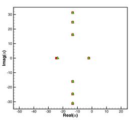
Fig.7, Eigenvalues at 800Hz for plug flow (square) and shear flow with turbulent boundary layer (triangle). Mach number: 0.452, boundary layer thickness: 1”, duct radius: 62.33”, azimuthal mode number m=22, cut-on frequency for the 1st radial mode of the plug flow: 740.6Hz.
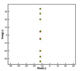
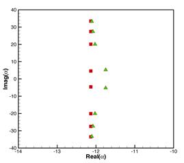
Fig.8,
Eigenvalues at 730Hz for plug flow (square) and shear flow with turbulent
boundary layer (triangle). Mach number: 0.452, boundary layer thickness: 1”,
duct radius: 62.33”, azimuthal mode number m=22,
cut-on frequency for the 1st radial mode of the plug flow: 740.6Hz.
[Real(![]() ) in the right figure is rescaled to show the difference.]
) in the right figure is rescaled to show the difference.]
A numerical integration method
can also be used.