Sound Generation from Vortex Sheet Instability

Hongbin Ju

Department of Mathematics

Florida State University, Tallahassee, FL.32306

www.aeroacoustics.info

Please send comments to: hju@math.fsu.edu

When two parallel flows meet, a free shear layer with velocity adjustment is formed (Fig.1). If shear layer thickness d is small, the flow may be unstable subject to even very small disturbances. This is the Kelvin-Helmholtz Instability. It has been discussed in many books (Landau and Lifshitz1959, Batchelor1973, etc). Here we will give the details of the solution and explain the physical meaning of the instability. It will be shown that under the disturbance, the initial uniform vorticity will redistribute itself and concentrated vortexes will be formed. During this process, pressure fluctuation occurs and sound wave is produced as the by-product.

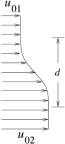
Fig.1, Shear layer between two flows.

Vortex Sheet Model

To simplify the problem, we assume d is very small compared to wavelengths of disturbances. The flow can then be modeled as two uniform flow regions (regions I and II) joined at an interface of discontinuity, shown in Fig.2. The flow directions are parallel to the interface. It is assumed there is no flow across the interface. According to cht21.doc (Wave Interactions at Surface of Discontinuity), this interface is a surface with tangential discontinuity. Across the interface, velocity and density can be discontinuous, but pressure must be continuous:

, , . (1)

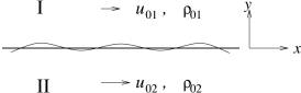
Fig.2, Vortex sheet model.

The two regions are vorticity free. Vorticity is uniformly distributed on the interface because of the velocity jump. The interface is therefore called vortex sheet. To quantify the vortex sheet, define circulation per unit length as (refer to Fig.3):

.

According to Stokesπ Theorem, circulation around ABCD is the total vorticity in rectangular area ABCD. Therefore represents the vortex strength of the vortex sheet.

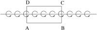
Fig.3, Circulation of the vortex sheet.

Let's use subscripts 1 and 2 denote the variables in region I and II respectively. One can show that:

. (2)

The vortex strength equals to the velocity jump across the vortex sheet. For the mean flow:

. (3)

Acoustic Solution and Dispersion Equation

The normal modes of linear Euler equations in a uniform flow region (I or II) have been given in cht1.doc (Waves in Uniform Flow on Half Plane). Entropy and vorticity waves can be uniquely determined from Eqs. (37)~(40), and Eqs. (45)~(48) in cht1.doc when two boundary conditions at upstream boundary are set. Acoustic waves can be computed from Eqs.(22)~(25) when boundary conditions are set at and in region I, and and in region II. For the problem in this section, there are no vorticity and heat waves from the upstream boundary, and there are no sound waves propagating towards the interface from . The disturbance only comes from the interface. Therefore there are only acoustic waves in regions I and II. According to Ch1t.doc, by assuming this form of solution:

, (4)

the acoustic solutions in region I and II are:

, (5)

, (6)

, (7)

and,

, (8)

, (9)

. (10)

The mean flows are assumed to be subsonic. and are assumed totally independent if there is no boundary. However, to meet the boundary conditions at the interface, these parameters must satisfy some relations. It becomes an eigenvalue problem due to the boundary conditions. ( or ) is determined by Eq.(26) in Ch1t.doc when is real. It will become clear that is complex for real for the vortex sheet problem. Therefore the branch cuts for in Cht1.doc (Eq.26 and Fig.1) are no longer applicable. We will discuss how to compute later.

When disturbed, the interface is at . The amplitude of the disturbance is assumed small, and the disturbed interface is still a surface of tangential discontinuity. According to cht21.doc (Wave Interactions at Surface of Discontinuity), two boundary conditions must be satisfied at the interface . The first is the kinematic boundary condition, i.e, the continuity of displacement of the vortex sheet on both sides. Then,

, , (11)

or,

, . (12)

From Eqs.(7), (10) and (12), we have:

and . (13)

With Eq.(13), one can express solutions in Eqs.(5)~(10) in terms of .

The second boundary condition at the interface is the dynamic boundary condition:

. (14)

From (5), (8) and (14), we have

. (15)

From Eq.(13) and Eq.(15), we obtain:

. (16)

Due to the interface boundary conditions, wave number and frequency are no longer independent variables. For each wave number , there are specific frequencies . Eq. (16) is called the dispersion equation.

Now we need to discuss the computation of ( or ) for complex . is determined by (Eq.19 in cht1.doc):

. (17)

, , .

We will choose appropriate branch cuts of on -plane to ensure . Then

(18)

will always have nonnegative imaginary part: (Fig.4). The branch cuts satisfy: , or,

. (19)

The two branch cuts are shown by solid wiggle lines in Fig.4. They approach asymptotically to the vertical line . On the branch cuts is real and the wave is a purely propagating wave. In Fig.4 extended from the branch cuts are dashed lines at which . Eq.(19) is also satisfied along these dashed lines, and they approach asymptotically to horizontal line . On these dashed lines is purely imaginary, representing purely spatially damped waves in y direction. All other waves with not on the branch cuts and the dashed lines are spatially damped propagating waves.

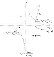
Fig.4, Branch cuts for .

Unstable Waves/Instability

For a simple wave of the form , a dispersion equation such as Eq.(16) relates wave number and frequency:

. (20)

From this dispersion equation, can be solved in terms of :

. (21)

There may be multiple solutions of . If one or more of for real are complex and have positive imaginary parts (), then the simple wave is unstable for this . Instability occurs if there are unstable waves in the system. The unstable simple wave has spatially periodic structure of infinite extent. Its amplitude grows to infinity as at every fixed point in space.

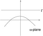
Fig.5, Contour of complex for real .

In actual situations, it is very rare there exists a disturbance with a periodic structure extent infinitively in space. A disturbance is more likely to be a pulse in space with finite spatial extent. The pulse can be represented by superposition of simple waves with real wave numbers. If in a range of , has positive imaginary part as in Fig.5, simple waves in this range are unstable and thus excited. Amplitudes of these waves will grow in time at every point in space. However, the composed disturbance (the pulse) has two distinct scenarios. One is that the pulse may grow at every fixed spatial point. This is called absolute instability. The other is that the amplitude of the pulse at any fixed point eventually decreases as . The reason is that the instability is convected away. This is called convective instability or spatial amplifying waves.

To investigate the instability evolvement of a pulse, the Laplace Transform on t must be employed. (Fourier Transform or normal mode method will not work.) Laplace transform is powerful in investigating the initial stage of unstable waves. The asymptotic response as can also be obtain from this method.

For the vortex sheet instability, the inverse Fourier-Laplace transform gives the pressure in region I:

. (22)

There are two ways for this Inverse Transform. One is to integrate first. If the disturbance at the interface is:

, (23)

then the sound pressure in region I is:

. (24)

(If there are multiple solution of from the dispersion equation (16), in the above equation should be the sum of integrals for all the .) is an entire function of . The limiting value of the integral as is determined by:

. (25)

The integral path is the contour of when is real as in Fig.5. If there is a saddle point where

(26)

in the area enclosed by and the real -axis, the integration will diverge as . This is the absolute instability. is the group velocity of a pulse. Eq.(26) means absolute instability happens when the group velocity is zero. The energy of instability waves do not propagate away. If , the instability waves will propagate away. At each spatial point the wave will decay eventually. This is convective instability. (Briggs1964, Tam class note)

Integration in Eq.(22) can also be carried first on :

. (27)

By pushing towards a little below the real -axis, one can investigate the sinusoidal steady-state response of the waves. During this process if a pole on the complex -plane move across the real -axis, the wave is a amplifying wave. Therefore it is the characteristics of (Eq.(21)) that determines if this wave is amplifying wave or evanescent wave, or absolute instability. Amplifying waves are also called spatial instabilities. Solution in terms of real from dispersion relation Eq.(20) gives the instability growth rate :

. (28)

The two inverse transform ways should have the same results. An amplifying wave in spatial instability in the second method is basically the same type as the convective instability of temporal instability in the first method.

No matter which method is used, the most critical thing is the dispersion equation in the form of for real , Eq.(21), and group velocity, Eq.(26) . If has positive imaginary part, the pulse will be unstable. If the group velocity is zero, then it is absolute instability. Otherwise, it is a convective instability/amplifying wave. Dispersion equations can be found using the normal mode method.

Vortex Sheet Instability

The characteristics of the vortex sheet instability hinges on in terms of real from dispersion relation Eq.(16). It is rather complicated to deal with Eq.(16) for compressible flows. Here we first consider incompressible flows. According to Cht1.doc (Waves in Uniform Flow on Half Plane) Eq.(28), for incompressible flows on both regions, and are pure imaginary number:

. (29)

The effect of the disturbance is only local to the interface. Eq.(16) can be simplified to:

, where density ratio . (30)

Temporal Instability

On solving in terms of real from Eq.(30), one has:

, , . (31)

Without loss of generality, from now on we will assume and . Then the solution represents a right-going wave with phase speed:

, (32)

which is density weighted average velocity of the two mean flows. When positive is taken in (31), , the amplitude of the wave grows exponentially at the rate of . The vortex sheet is unstable subject to disturbance with any wave number. Since

, (33)

The instability is convective instability.

The physical meaning of the vortex sheet instability can be explained by examining the disturbance circulation per unit length Eq.(2) (Batchelor1973):

. (34)

Vorticity varies sinusoidally with a phase difference to displacement . The total disturbance vorticity at the interface is zero. The pressure at the interface is:

. (35)

If we simply assume the same density on both sides, , then,

. (36)

The phase of circulation is greater than that of displacement as in Fig.6. The disturbance redistributes vorticity instead of generating new vorticity. There are two types of points for . One, denoted by A, is the type of points where and . Near these points, the vortex rotates anticlockwise and is swept by convection toward these points and accumulated. The other type, denoted by B, is the type of points where and . Near these points, the vortex rotates in clockwise direction and is swept away from these points. Thus the result of the disturbance is the concentration of vorticity and formation of discrete vortexes near type A points. The vortexes will further enhance the convection and make the vorticity more concentrated, leading to exponential growth of the disturbance in time.

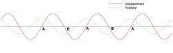
Fig.6, Displacement and circulation at the interface for the unstable wave.

Pressure at the interface Eq.(35) is when :

. (37)

It is exactly out of phase with vorticity. The lowest pressure is at the vortex center.

The Kelvin-Helmholtz instability sometimes is explained by the wavy wall analogy (Ackeretπs explanation, c.f. Tam&Hu1989). Look at the flow in the frame moving with the phase velocity (Eq.(32)) of the instability wave as in Fig.7. The vortex sheet can be seen as a wavy wall. First we assume the wavy wall is steady (doesnπt change the shape). The pressure at both sides are indicated by + and ≠ on these troughs and crests to show high or low pressure. Since one crest on one side is a trough on the other side, there is net pressure imbalance across the interface. The interface is not exactly the same as a wavy wall in that the interface self can deform under this pressure imbalance. The deformation makes the pressure imbalance more appreciable. This causes the instability.

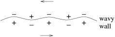
Fig.7, Wavy wall model of vortex sheet instability.

Another possible solution in Eq.(31) is . The circulation per unit length:

. (38)

The vorticity variation has phase lag to displacement . Points B in Fig.6 are now the center of accumulation. The subsequent motion would be to rotate around B in anti-clockwise and the vorticity is swept away from B instead of towards it. Then the disturbance would diminish exponentially. That means this solution is unlikely to manifest itself naturally.

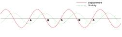
Fig.8, Displacement and circulation at the interface for the stable wave.

If , circulation produced by baroclinic vorticity production mechanism is:

. (39)

Obviously there is density gradient in y-direction, so if there will be vorticity production:

. (40)

From which we know that the vorticity is no longer just redistributed itself as in the case, although the total vorticity produced baroclinically is zero. The minimum pressure is no longer exactly at the vortex centers.

Spatial Instability

Kelvin-Helmholtz instability is convective instability. If the disturbance is generated in a local region, such as the jet from a nozzle exhaust, the convective instability will reveal itself as a spatially amplifying wave. From Eq.(30), the wave number in terms of frequency is:

. (41)

There are two poles on complex -plane. The characteristics of the two poles should be investigated using Briggsπ method by assuming with a very large imaginary part. When has very large imaginary part, both the poles are on the up half of the -plane. As the imaginary part of approaches zero, the pole with negative sign before i in Eq.(41) moves across the interface to the lower half of the -plane. This pole corresponds to an amplifying wave (spatial instability). The spatial growth rate is determined from the imaginary part of :

. (42)

Suppose , and (as in a jet),

. (43)

Then the spatial growth rate is (Anand):

. (44)

We assumed incompressible flows on both sides of the interface. In this situation the disturbance only propagates along the interface. It decays exponentially in normal direction of the interface. Therefore the disturbance can not propagate to the far field. For compressible flows, it is rather complicated to solve in terms of from dispersion equation (16). From Fig.4, except at one point where the dashed line intersects with the real -axis, all real corresponds to a damped propagating wave, although waves with of large absolute values are highly damped. That means for compressible flows the disturbances from vortex sheet instability propagate away to the far field.

In the vortex sheet model viscosity is ignored. The instability is believed to be due to the inflexion point in the velocity profile. Kelvin-Helmholtz Instability is inflexion instability. Vortex sheet model can provide good estimate of phase speed of the instability wave, Eq.(32). But for purpose of calculating the growth rate of the wave, Eq.(44), a finite thickness model is necessary. In some cases, the wave is neutral (zero growth rate) in the vortex sheet model, but in finite thickness model the growth rate is finite. In the vortex sheet model, Kelvin-Helmholtz Instability is a convective instability, however, if finite thickness model is used, it is possible the K-H instability is an absolute instability.