Low Mach Number Flow Noise:
Flow as the Quadrupole Source
Hongbin Ju
Department of Mathematics
Florida State University, Tallahassee, FL.32306
www.aeroacoustics.info
Please send comments to: hju@math.fsu.edu
In a uniform flow, linear waves of vorticity, sound and heat are independent. They interact with each other only at boundaries. When the flow is not uniform, or disturbances in the flow are not small, different waves will interact by scattering and/or nonlinearity: one type of wave can grow, be generated or dampened by other types of waves.
It
is difficult to analyze wave interactions in a nonlinear nonuniform flow. In
this chapter we will discuss a simple case of nonlinear interaction: the sound generation by a compact vortical flow
with low Mach number M, shown by Fig.1.
The flow moves at typical speed ![]() which is much
smaller than sound speed a.
During one cycle of the typical oscillation with period T, the ratio of distance l traveled by the flow to sound wavelength
which is much
smaller than sound speed a.
During one cycle of the typical oscillation with period T, the ratio of distance l traveled by the flow to sound wavelength ![]() is
is ![]() . Because Mach number M is small, the two lengths are disparate:
. Because Mach number M is small, the two lengths are disparate: ![]() . On flow length scale l, the flow in its low order M expansion is vortical and incompressible. On sound wavelength scale
. On flow length scale l, the flow in its low order M expansion is vortical and incompressible. On sound wavelength scale ![]() , the flow is irrotational in its low order M expansion. That means the short and very long lengths
are only weakly coupled in the flow and sound regions. The physical explanation
of this weak coupling is, during one cycle of the flow parameter, the sound
wave oscillates many cycles so its net effect is almost cancelled; on the other
hand, the slowly varying flow is almost constant over one cycle of the sound
oscillation. (Crighton, et.al.1992, p.209) Therefore, one may only need to solve
an incompressible flow in the flow region and solve the sound wave equation in
the sound wave region. The two solutions are then coupled in an overlap region.
This coupling is fulfilled only mathematically. There is no physical solution
in the overlap region. In the final solution the incompressible flow acts as a
quadrupole source to the far sound field, which is the same as in the
Lighthillπs Analogy Theory.
, the flow is irrotational in its low order M expansion. That means the short and very long lengths
are only weakly coupled in the flow and sound regions. The physical explanation
of this weak coupling is, during one cycle of the flow parameter, the sound
wave oscillates many cycles so its net effect is almost cancelled; on the other
hand, the slowly varying flow is almost constant over one cycle of the sound
oscillation. (Crighton, et.al.1992, p.209) Therefore, one may only need to solve
an incompressible flow in the flow region and solve the sound wave equation in
the sound wave region. The two solutions are then coupled in an overlap region.
This coupling is fulfilled only mathematically. There is no physical solution
in the overlap region. In the final solution the incompressible flow acts as a
quadrupole source to the far sound field, which is the same as in the
Lighthillπs Analogy Theory.
The
mathematic tool for this analysis is the perturbation method. We first assume
the flow is incompressible (![]() ). An incompressible flow is localized. Then a small compressibility
is admitted. Admission of compressibility has two effects. First, the flow
energy can propagate away in the form of compressible waves (sound) from the
local flow region. Second, there is time lag between the flow and its generated
sound. Mach number M is the expansion
parameter. It is the ratio of two lengths. The disparity of the two length
scales implies that the low Mach number flow sound is a multiple scale problem,
and the perturbation will be singular instead of regular (Dyke1975, p.80: a
perturbation solution is uniformly valid in the space and time coordinates
unless the perturbation quantity is the ratio of two lengths or two times).
). An incompressible flow is localized. Then a small compressibility
is admitted. Admission of compressibility has two effects. First, the flow
energy can propagate away in the form of compressible waves (sound) from the
local flow region. Second, there is time lag between the flow and its generated
sound. Mach number M is the expansion
parameter. It is the ratio of two lengths. The disparity of the two length
scales implies that the low Mach number flow sound is a multiple scale problem,
and the perturbation will be singular instead of regular (Dyke1975, p.80: a
perturbation solution is uniformly valid in the space and time coordinates
unless the perturbation quantity is the ratio of two lengths or two times).
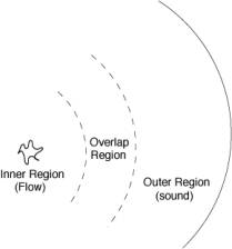
Fig.1, Sound generation by low Mach number compact flow.
There are two different singular perturbation methods. Landau and Lifshitz first used the Matched Asymptotic Expansion (MAE) to compute sound from a small pulsating and oscillating body. Crow1970, Obermeier1985 extended this MAE method to low Mach number flow sound problem. Different length scales are used in the near field flow region and the far field sound region. Regular expansions are developed based on their local length scales in different regions. The two expansions are then matched in the overlap region to form a composite solution.
The other
method is Multiple Scale Method. One may
choose one time scale and two length scales (l and ![]() ) in the analysis as in Fortenbach&Munz2003. Since for
the same distance, the time spent by the sound wave is much shorter than that
by the flow, one may also use one length scale and two time scales in the Multiple
Scale method as in M¸ller1999.
) in the analysis as in Fortenbach&Munz2003. Since for
the same distance, the time spent by the sound wave is much shorter than that
by the flow, one may also use one length scale and two time scales in the Multiple
Scale method as in M¸ller1999.
MAE method similar to Crow1970 will be employed here. The following are the equations for inviscid, non-heat-conducting flow used in this chapter:
![]() ,
(1)
,
(1)
![]() ,
(2)
,
(2)
![]() .
(3)
.
(3)
Inner Expansion
Success
of MAE depends on choosing right scales in the region analyzed. Different
choice of scales gives different results. In the flow region, the flow is fully
characterized by typical eddy speed ![]() (velocity scale),
typical eddy size l (length scale), and
time scale
(velocity scale),
typical eddy size l (length scale), and
time scale ![]() . From continuity equation (1), density scale has no
significance. Generally we use density in the far field
. From continuity equation (1), density scale has no
significance. Generally we use density in the far field ![]() as the density
scale. From momentum equation (2), the relative scale of pressure to that of
density is critical for the analysis. However, the appropriate pressure scale
can't be found from the momentum equation. It can be found from isentropic
equation (3). It is straightforward to choose pressure in the far field
as the density
scale. From momentum equation (2), the relative scale of pressure to that of
density is critical for the analysis. However, the appropriate pressure scale
can't be found from the momentum equation. It can be found from isentropic
equation (3). It is straightforward to choose pressure in the far field ![]() as the scale. Just
for convenience, we usually choose
as the scale. Just
for convenience, we usually choose ![]() (sound
speed
(sound
speed ![]() ) as the pressure scale. Then the dimensionless equations
are:
) as the pressure scale. Then the dimensionless equations
are:
![]() ,
(4)
,
(4)
![]() ,
, ![]() ,
(5)
,
(5)
![]() . (6)
. (6)
All variables in (4)~(6) and hereafter are dimensionless quantities unless specified.
Let's try the regular expansion series:
![]() ,
(7)
,
(7)
![]() ,
(8)
,
(8)
![]() .
(9)
.
(9)
Substituting them into (4)~(6) and equating the terms of like powers of M, we have:
![]() equations:
equations:
![]() ,
, ![]() ,
, ![]() .
(10)
.
(10)
The
general solution of ![]() is
is ![]() , which should be determined by matching it to the outer
expansion in the overlap region. From physics intuition, it should be the
atmospheric pressure in the far field
, which should be determined by matching it to the outer
expansion in the overlap region. From physics intuition, it should be the
atmospheric pressure in the far field ![]() . Therefore,
. Therefore,
![]() ,
, ![]() , and
, and ![]() .
(11)
.
(11)
![]() equations:
equations:
![]() ,
, ![]() ,
, ![]() .
(12)
.
(12)
The
same argument as in ![]() equations indicates:
equations indicates:
![]() ,
, ![]() ,
, ![]() .
(13)
.
(13)
(11) and (13) have similar properties. There is no
advantage to separate these two orders of equations (Crow1970, M¸ller1999,
Eldredge2002). Therefore, ![]() and
and ![]() order variables can be combined. The proper expansion
series should be:
order variables can be combined. The proper expansion
series should be:
![]() ,
(14)
,
(14)
![]() ,
(15)
,
(15)
![]() .
(16)
.
(16)
Now ![]() ,
, ![]() , and
, and ![]() are variables of
are variables of
![]() and
and ![]() orders, instead of variables only of
orders, instead of variables only of ![]() order as in (7)~(8).
order as in (7)~(8).
Substituting (14)~(16) into (4)~(6), we have:
![]() +
+![]() equations:
equations:
![]() ,
, ![]() ,
, ![]() .
(17)
.
(17)
The same argument as for (11) brings to:
![]() ,
, ![]() ,
, ![]() .
(18)
.
(18)
In this order the flow is solenoidal (dilation free).
![]() equations:
equations:
![]() ,
(19)
,
(19)
![]() ,
(20)
,
(20)
![]() .
(21)
.
(21)
From (18) we know in the limit of low compressibility, pressure converges to a constant thermodynamic background pressure. When small compressibility is admitted, from equations (18) and (20), we can form the following complete system of equations:
![]() ,
(22)
,
(22)
![]() .
(23)
.
(23)
These
are the well known incompressible flow equations. They are actually the low
Mach number flow equations. Velocity field is solenoidal. We will use ![]() instead of
instead of ![]() in the
equations. Taking divergence on both sides of (23), we have the Poisson
equation about pressure:
in the
equations. Taking divergence on both sides of (23), we have the Poisson
equation about pressure:
![]() .
(24)
.
(24)
Its solution in three dimensions if ![]() is known is:
is known is:
![]() ,
(25)
,
(25)
where![]() ,
, ![]() with
with ![]() fixed. Any
harmonic solution J (solution of
fixed. Any
harmonic solution J (solution of ![]() ) can be added to
) can be added to ![]() to form another
solution. But J is analytical and
will grow algebraically in the far field (Crighton, et.al.1992). Thus J
should not be included in the solution.
to form another
solution. But J is analytical and
will grow algebraically in the far field (Crighton, et.al.1992). Thus J
should not be included in the solution.
From
(18) and (25), to second order ![]() , the formal solution of pressure in the flow region is:
, the formal solution of pressure in the flow region is:
![]() .
(26)
.
(26)
Solutions
(25) and (26) are only formal since ![]() has to be solved
together with
has to be solved
together with ![]() from incompressible
equations (22) and (23).
from incompressible
equations (22) and (23). ![]() is called hydrodynamic
pressure. Hydrodynamic pressure appears in
incompressible equation (23) to establish the divergence-free velocity
is called hydrodynamic
pressure. Hydrodynamic pressure appears in
incompressible equation (23) to establish the divergence-free velocity ![]() . Associated with
. Associated with ![]() is hydrodynamic
density
is hydrodynamic
density ![]() [Eq.(21)] and
second order velocity
[Eq.(21)] and
second order velocity ![]() [Eq.(19)].
[Eq.(19)]. ![]() is not
necessarily dilation free. That means
is not
necessarily dilation free. That means ![]() may compress the
fluid element, although in this low order [
may compress the
fluid element, although in this low order [![]() ] there is no sound,
Eq.(24).
] there is no sound,
Eq.(24).
An acoustic/viscous splitting numerical scheme can be established based on this asymptotic analysis. One may use the next asymptotic series:
![]() ,
(27)
,
(27)
![]() ,
(28)
,
(28)
![]() .
(29)
.
(29)
![]() ,
, ![]() ,
, ![]() and
and ![]() have small
length scale l. They are solved from
incompressible equations (22)&(23) and equations (21)&(19) on a fine
grid system. Substitute expansions (27)~(29) into the N.S. equations and
subtract the incompressible equations from them to obtain a set of equations for
have small
length scale l. They are solved from
incompressible equations (22)&(23) and equations (21)&(19) on a fine
grid system. Substitute expansions (27)~(29) into the N.S. equations and
subtract the incompressible equations from them to obtain a set of equations for
![]() ,
, ![]() , and
, and ![]() . These equations are acoustic equations. Since only the long length scale, sound wavelength,
exists in the acoustic equations, they can be solved on a coarse grid system.
By splitting the incompressible flow and the sound waves, the singularity due
to length scale disparity is removed. A similar acoustic/viscous splitting
numerical scheme was proposed by Hardin&Pope1994, in which
. These equations are acoustic equations. Since only the long length scale, sound wavelength,
exists in the acoustic equations, they can be solved on a coarse grid system.
By splitting the incompressible flow and the sound waves, the singularity due
to length scale disparity is removed. A similar acoustic/viscous splitting
numerical scheme was proposed by Hardin&Pope1994, in which ![]() is not solved in
the incompressible flow.
is not solved in
the incompressible flow.
Outer
Expansion
In
the sound region, the appropriate length scale is sound wavelength ![]() . Use
. Use ![]() as the new
length scale to define the dimensionless coordinate:
as the new
length scale to define the dimensionless coordinate:
![]() .
(30)
.
(30)
Eq.(30)
is a stretching transformation of the coordinate. The sound is generated by the
fluid flow, therefore the inner and outer regions have the same time scale: ![]() .
. ![]() is the density
scale and
is the density
scale and ![]() the pressure
scale. We may still use
the pressure
scale. We may still use ![]() as the velocity
scale. However we may have a better choice. From the
as the velocity
scale. However we may have a better choice. From the ![]() momentum equation of the inner
expansion,
momentum equation of the inner
expansion, ![]() (on the inner
expansion scales), then the pressure fluctuation in dimensional form is
(on the inner
expansion scales), then the pressure fluctuation in dimensional form is ![]() . As we know for sound waves,
. As we know for sound waves, ![]() (
(![]() is the acoustic velocity). Which means the acoustic velocity
is in the order of
is the acoustic velocity). Which means the acoustic velocity
is in the order of ![]() , which seems to be a better choice for velocity scale in the
outer region:
, which seems to be a better choice for velocity scale in the
outer region: ![]() . Then the dimensionless equations in the outer region are:
. Then the dimensionless equations in the outer region are:
![]() , (31)
, (31)
![]() , (32)
, (32)
![]() .
(33)
.
(33)
The next regular expansion series are used:
![]() , (34)
, (34)
![]() ,
(35)
,
(35)
![]() . (36)
. (36)
We have:
![]() +
+![]() equations:
equations:
![]() ,
, ![]() ,
, ![]() . (37)
. (37)
The ![]() solutions are:
solutions are:
![]() ,
, ![]() .
(38)
.
(38)
![]() equations:
equations:
![]() ,
, ![]() ,
, ![]() . (39)
. (39)
From the momentum equation in (39), one has:
![]() .
.
In the far field there is no vorticity initially, therefore the velocity field is vorticity free in this order:
![]() .
(40)
.
(40)
The wave equation is obtained from equations in (39):
![]() .
(41)
.
(41)
![]() equations:
equations:
![]() ,
, ![]() ,
, ![]() . (42)
. (42)
The solutions are:
![]() .
(43)
.
(43)
![]() equations:
equations:
![]() ,
(44)
,
(44)
![]() ,
(45)
,
(45)
![]() .
(46)
.
(46)
In
this order vorticity ![]() is not
necessarily zero.
is not
necessarily zero.
![]() equations:
equations:
![]() , (47)
, (47)
![]() ,
(48)
,
(48)
![]() . (49)
. (49)
From
(48), ![]() .
.
The wave equation is:
![]() . (50)
. (50)
Here we will only discuss the solution to ![]() wave equation (50) because it is the
term which will match the inner expansion. The general solution to this wave
equation is composed of monopoles, dipoles, quadrupoles, and even higher order
components. But only the quadrupole is needed for matching to the inner
solution:
wave equation (50) because it is the
term which will match the inner expansion. The general solution to this wave
equation is composed of monopoles, dipoles, quadrupoles, and even higher order
components. But only the quadrupole is needed for matching to the inner
solution:
![]() , where
, where ![]() .
(51)
.
(51)
Therefore, pressure in the sound field is:
![]() . (52)
. (52)
Matching
Both
the inner and outer expansions are the approximations to the same function, but
just in different regions. They have to match with each other in the overlap
region. There are two matching methods: Intermediate Matching Principle and
Asymptotic Matching Principle (Crighton, et.al. 1992, Van Dyke1975,
Holmes1995). We will use Intermediate Matching Principle here. In this method,
the two expansions match in an overlap region. As ![]() , the overlap region is the far field for the inner region,
but a near field for the outer expansion. To describe this region
mathematically, a new coordinate system is introduced:
, the overlap region is the far field for the inner region,
but a near field for the outer expansion. To describe this region
mathematically, a new coordinate system is introduced:![]() .
. ![]() is chosen so
that as
is chosen so
that as ![]() when keeping
when keeping ![]() fixed,
fixed,
![]() ,
, ![]() . (53)
. (53)
One
may choose ![]() ,
, ![]() . In the new coordinate system,
. In the new coordinate system,
 ,
(54)
,
(54)
![]() .
.
Inner solution (26) can be written in the new coordinate system as:
 . (55)
(Note
that the scale of ![]() is still l.)
is still l.)
Outer solution (52) is rewritten as:
 .
(56)
.
(56)
Matching
the terms with ![]() in (55) and
(56), we have:
in (55) and
(56), we have:
![]() .
(57)
.
(57)
Final
Solutions
Now
we summarize the final solutions with scales: length l, velocity ![]() , time
, time ![]() , density
, density ![]() , and pressure
, and pressure ![]() .
.
Inner solution:
 ,
(58)
,
(58)
![]() , (59)
, (59)
![]() ; (60)
; (60)
![]() ,
(61)
,
(61)
![]() , (62)
, (62)
![]() ,
(63)
,
(63)
![]() . (64)
. (64)
Outer solution:
![]() , (65)
, (65)
![]() ,
(66)
,
(66)
 ;
(67)
;
(67)
 , (68)
![]() ,
(69)
,
(69)
![]() .
(70)
.
(70)
Acoustic Analogy
of the Low Speed Flow Sound
From
sound wave equation (50) and solution (68), the equivalent inhomogeneous wave
equation in the sound field is:
![]() , or (71)
, or (71)
![]() . (72)
. (72)
In dimensional form, inhomogeneous wave equation (72) is (the same variable names are used):
![]() . (73)
. (73)
The nonlinear
incompressible flow in the near field acts as a quadrupole source driving the far
field acoustic field. Strength of the quadrupole source is ![]() , which is the Lighthill stress tensor in Lighthillπs Analogy Theory. From Eq.(24),
, which is the Lighthill stress tensor in Lighthillπs Analogy Theory. From Eq.(24),
![]() .
(74)
.
(74)
![]() is the
hydrodynamic pressure in the near field.
is the
hydrodynamic pressure in the near field. ![]() represents the
relative value of
represents the
relative value of ![]() at one point
compared to the average pressure around this point.
at one point
compared to the average pressure around this point. ![]() means
means ![]() is the local
minimum, otherwise it is the local maximum. Therefore, the sound source is the
pressure at one point relative to the averaged pressure of its neighbor caused
by the turbulent eddies.
is the local
minimum, otherwise it is the local maximum. Therefore, the sound source is the
pressure at one point relative to the averaged pressure of its neighbor caused
by the turbulent eddies. ![]() is called jetlets
by Ribner.
is called jetlets
by Ribner.
The
same result can also be obtained by weakly nonlinear analysis.