Acoustic
Energy and Intensity
Hongbin Ju
www.aeroacoustics.info
hju0308@gmail.com
In this section we discuss acoustic energy, acoustic intensity, and their components. Emphasis will be played on the definition of acoustic intensity, which is the acoustic energy flux passing through a unit area in unit time. It is straightforward to define an instantaneous acoustic intensity from the energy equation. However, in practical problems the major concern is time averaged energy flux. Terms with zero time average should be ignored. Terms that make no contribution to mean energy should also be ignored. Only terms with even orders of magnitude in the expansion of instantaneous acoustic intensity are important and should be kept in the definition of the acoustic intensity.
Ideal gas (![]() ) with isentropic process (
) with isentropic process (![]() ) is assumed. Linear disturbances
are only generated by acoustic waves.
) is assumed. Linear disturbances
are only generated by acoustic waves.
Balance of Acoustic Energies
Decomposition of Variables
Variables for undisturbed flows
are defined with subscript ‘0’, such as, ![]() ,
, ![]() ,
, ![]() . Any variable in a disturbed flow is decomposed into a time
averaged component and a fluctuation component:
. Any variable in a disturbed flow is decomposed into a time
averaged component and a fluctuation component:
![]() , (1)
, (1)
![]() ,
,
![]() ,
, ![]() .
.
Generally for linear disturbances,
![]() [hj1] .
(2)
[hj1] .
(2)
For a product of two variables, such as ![]() ,
,
![]() .
(3)
.
(3)
Euler Equations
Euler equations and their forms with time averaged and fluctuation variables are as following.
The continuity
equations are:
![]() , (4)
, (4)
![]() . (5)
. (5)
The momentum
equations are:
![]() , (6)
, (6)
 . (7)
. (7)
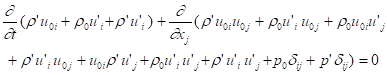
The conservative form of the energy equation is:
![]() .
(8)
.
(8)
The total energy in unit fluid volume
![]() (9)
(9)
has two components: the internal energy![]() and the kinetic energy
and the kinetic energy ![]() . Since only acoustic perturbations are assumed, the internal
energy is the acoustic potential energy, and the kinetic energy is translational, not rotational,
kinetic energy. The instantaneous
acoustic intensity
. Since only acoustic perturbations are assumed, the internal
energy is the acoustic potential energy, and the kinetic energy is translational, not rotational,
kinetic energy. The instantaneous
acoustic intensity
![]() (10)
(10)
also has two components: energy
convection intensity ![]() and energy production
and energy production ![]() (work done by pressure).
(work done by pressure).
For a time steady process, the time average of the total energy in the volume is constant. Therefore the time averaged equation of Eq.(8) is:
![]() . (11)
. (11)
The time averaged total energy flux across the enclosing surface of a fluid element is zero.
Acoustic intensity Eq.(10) in this form has never been used. We will show that the acoustic intensity has many components. Some of them can be ignored and a simplified form of acoustic intensity can be defined.
Acoustic Energy Components and Their Equations
For an isentropic flow,
![]() , or
, or ![]() , (12)
, (12)
and the internal energy density is:
![]() .
(13)
.
(13)
For the isentropic process, the continuity and momentum equations (5)&(7) with equation of state (12) is a complete system for solving the equations. Energy equation (8) can be derived from equations (5)&(7). It is not needed for solving the sound field but very useful for energy balance analyses.
With the isentropic relation, continuity equation (5) can be rewritten as:
![]() . (14)
. (14)
This equation shows the balance of the internal energy. The time rate of
internal energy is equal to the internal energy convected
into the fluid element ![]() , plus the work
, plus the work ![]() done by the pressure
on the fluid element by changing its volume.
done by the pressure
on the fluid element by changing its volume.
Multiplying both sides of momentum equation (7) by ![]() and making use of the
continuum equation (4), we have:
and making use of the
continuum equation (4), we have:
![]() . (15)
. (15)
This equation shows the balance of the kinetic energy. The time rate of the kinetic
energy is the sum of its convection into the fluid (![]() ) and the work done by the net force on the movement of the
fluid volume (
) and the work done by the net force on the movement of the
fluid volume (![]() ).
).
Adding Eqs.(14) and (15) together one obtains the total energy equation (8).
Acoustic Intensity in Stationary Ideal Homogeneous Medium
We start with the simplest case:
quiescent uniform medium (![]() ).
).
Acoustic Energy Balance
Since pressure varies adiabatically with density (Eq.(12)), we have
![]() ,
,
i.e., ![]() , (16)
, (16)
![]() .
.
Therefore, the internal energy
![]() . (17)
. (17)
The zeroth,
first, and second orders of the internal energy fluctuations are
![]() ,
, ![]() , and
, and ![]() respectively.
respectively.
The kinetic energy to the second order is:
![]() .
(18)
.
(18)
The total acoustic energy fluctuation to the second order is:
![]() . (19)
. (19)
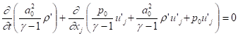
The acoustic energy equation to the 2nd order is:
 . (20)
Decomposition of Acoustic Energy and Acoustic Intensity
First order perturbations contribute nothing to the mean acoustic energy. It seems appropriate to define the time averaged acoustic intensity from Eq.(20) as
![]() .
(21)
.
(21)
We will show that the convection
intensity, ![]() , makes no contribute to the mean acoustic energy and
thus should be removed from definition.
, makes no contribute to the mean acoustic energy and
thus should be removed from definition.
Energy balance equation (20) can be separated into two equations about the internal energy such as Eq.(14) and the kinetic energy such as Eq.(15). To facilitate the definition of mean acoustic intensity, we decompose the energy equation based on the work done by the pressure on the fluid element:
![]() .
(22)
.
(22)
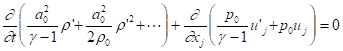
With continuity equation (5) and the uniform medium,
 . (23)
It is noted Eq.(23) looks similar but different from the perturbation form of internal energy equation (14)
 .
.
Eq.(23) is
basically the continue equation but it does reveals the balance of the first
order of internal energy ![]() in a quiescent uniform
flow. The time average of
in a quiescent uniform
flow. The time average of ![]() is zero.
is zero. ![]() has
no contribution to the mean acoustic energy although its time average is not
zero. Therefore, it should not be included in the definition of mean acoustic
intensity.
has
no contribution to the mean acoustic energy although its time average is not
zero. Therefore, it should not be included in the definition of mean acoustic
intensity.
Subtracting Eq.(23) from (20), we have:
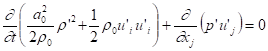 .
(24)
.
(24)
The time rate of the 2nd
order acoustic energy is due to the net work ![]() done by acoustic pressure
on acoustic velocity. Of the acoustic energy,
done by acoustic pressure
on acoustic velocity. Of the acoustic energy, ![]() is the internal energy
or acoustic potential-energy density,
generated by net pressure pushing the flow element
is the internal energy
or acoustic potential-energy density,
generated by net pressure pushing the flow element ![]() .
. ![]() is
the acoustic kinetic-energy density,
generated by pressure pressing the fluid element to change its volume
is
the acoustic kinetic-energy density,
generated by pressure pressing the fluid element to change its volume ![]() .
.
From equation (24), one can define the acoustic intensity as:
![]() ,
(25)
,
(25)
which is
the standard definition for stationary media. Note that this energy flux only
affects the second order energy fluctuation ![]() instead of the total
acoustic energy fluctuation
instead of the total
acoustic energy fluctuation ![]() . Since the time average of the first order
fluctuation internal energy
. Since the time average of the first order
fluctuation internal energy ![]() is zero, this definition makes more sense for energy
analyses.
is zero, this definition makes more sense for energy
analyses.
Acoustic Intensity with Mean Flow
Acoustic Energy Balance Equation
The total energy per unit volume of a mean flow is:
![]() . (26)
. (26)
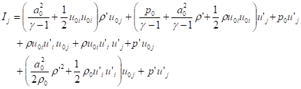
To the second order the acoustic energy fluctuation is:
![]() . (27)
. (27)
The time averages of first order terms are zero.
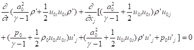
The acoustic energy balance equation is:
![]() ,
(28)
,
(28)
where
 . (29)
Decomposition of
Acoustic Energy in Uniform Mean Flow
For uniform ![]() and
and ![]() , continuity equation (5) can be rewritten as
, continuity equation (5) can be rewritten as
 . (30)
This reveals time rate of two
terms of the 1st order energy due to work ![]() done by the ambient pressure
on the acoustic velocity. The time average of this part of the energies is
zero. Although the time average of the second order term
done by the ambient pressure
on the acoustic velocity. The time average of this part of the energies is
zero. Although the time average of the second order term ![]() on the right hand side
is not zero, it contributes nothing to the mean acoustic energy. Therefore this
part of the energy flux should not be included in the acoustic intensity.
on the right hand side
is not zero, it contributes nothing to the mean acoustic energy. Therefore this
part of the energy flux should not be included in the acoustic intensity.
From momentum equation (7),
continuity equation (5) and uniform ![]() , we have the balance equation:
, we have the balance equation:
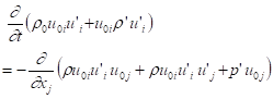 .
(31)
.
(31)
This part of energy balance is
due to work ![]() done by the acoustic
pressure on the mean velocity. The energy has a second order term with nonzero
time average.
done by the acoustic
pressure on the mean velocity. The energy has a second order term with nonzero
time average.
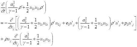
Subtracting Eq.(29) by (30) and (31), the equation for the rest of the acoustic energies is:
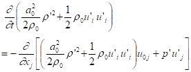 . (32)
Both energy terms are second order with nonzero time
average. It is due to work ![]() by the acoustic
pressure and the acoustic velocity.
by the acoustic
pressure and the acoustic velocity.
The three acoustic energy balance
equations, (30), (31), (32), are separated based on the separation of work ![]() .
.
Acoustic Intensity in
Uniform Mean Flow
Following the same logic as in the previous analyses for quiescent uniform media, based on Eqs.(31)&(32), the acoustic intensity in the j direction for a uniform mean flow can be defined as:
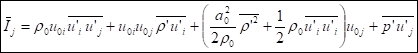 . (33)
All first order terms are averaged out. Third and higher
order terms are ignored. According to Lighthill
(p.11), in linear acoustics first order quantities are retained and quadratic
terms neglected in linear continuity and momentum equations, while in energy
equations, first order terms should be absent, most quadratic terms retained,
and cubic terms or above neglected. The only quadratic term absent is ![]() which does not
contribute to mean acoustic energy according to Eq.(30).
which does not
contribute to mean acoustic energy according to Eq.(30).
A similar definition was proposed in Cantrell&Hart 1964 Eq.(13) for isentropic uniform mean flows:
![]() . (34)
. (34)
This definition has been widely
accepted (Tester et.al.2004, Morfey1971, Möhring1971). According to Eq.(31) in cht1.doc, the time averaged acoustic potential
energy is equal to the acoustic kinetic energy: ![]() , with which, Eq.(34) and Eq.(33) are equivalent. The benefit
of using Eq.(34) instead of (33) is that it excludes
vortical energy if the disturbances have vortical component.
, with which, Eq.(34) and Eq.(33) are equivalent. The benefit
of using Eq.(34) instead of (33) is that it excludes
vortical energy if the disturbances have vortical component.
Acoustic Intensity in Nonuniform Mean Flow
Equations (30), (31) and (32) do not hold for a general nonuniform flow. From continuity equation (5), we have:
 . (37)
There is an extra term 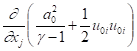 compared with Eq.(30) for uniform flows.
We may resort to Eq.(29) to define the acoustic intensity for a general mean flow as:
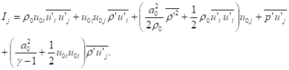 (40)
(40)
Quadratic term ![]() can no longer be
absent as for uniform flows in Eq.(33). Its
contribution to time averaged energy is zero only when the mean flow is
uniform.
can no longer be
absent as for uniform flows in Eq.(33). Its
contribution to time averaged energy is zero only when the mean flow is
uniform.
Applications of Acoustic Intensity
In this section we give an example of the application of acoustic
intensity (33) or (34) in hard wall circular duct.
From Eq.(11), the time averaged acoustic energy flux across an enclosed surface is:
![]() .
(41)
.
(41)
For a circular duct in Fig.1, we choose the enclosing surface shown by the shaded area. At cross section A, the sound power (sound energy across this section in unit time) is:
![]() .
(42)
.
(42)
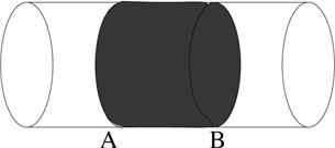
Fig1, Control surface in the circular duct.
Sound powers across section B, ![]() , and sound power across the duct wall,
, and sound power across the duct wall, ![]() , can be defined similarly. From Eq.(41),
we have:
, can be defined similarly. From Eq.(41),
we have:
![]() .
(43)
.
(43)
From the sound power distribution in the axial direction one can calculate the sound power absorbed by the duct wall. This is the base for liner duct analyses.
Sound Power in Axial Direction for Hard Wall Circular Duct
Dimensions used are: length: duct
diameter D, velocity: sound speed ![]() , density:
, density: ![]() , pressure:
, pressure: ![]() , energy flux:
, energy flux: ![]() , and sound power:
, and sound power: ![]() .
.
Acoustic intensity in the axial direction from (34) (Cantrell&Hart) is:
![]() . (44)
. (44)
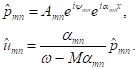
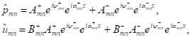
Assume the next form of the waves in the duct for circular frequency ![]() :
:
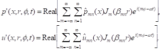 (45)
(45)
m, n are respectively the circumferential and radial mode numbers. mnth
mode will be used to indicate the mode with circumferential mode number m and radial mode number n. ![]() is the first kind
Bessel function. For hard wall,
is the first kind
Bessel function. For hard wall, ![]() is real.
is real.
By means of orthogonality of Bessel function, one can show that:
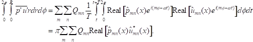 (46)
(46)
where * represents complex conjugate, and,
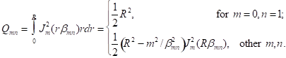 (47)
(47)
Similar equations hold for ![]() and
and ![]() .
.
Therefore, the total sound power is the sum of all sound powers calculated from each mnth mode:
![]() ,
(48)
,
(48)
![]() .
.
Note the sound power is the real part of the expression.
Next we will discuss the sound power for a single (m, n) mode.
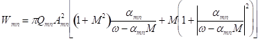
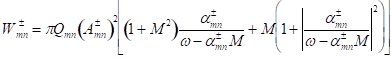
(m, n) Mode
in One Axial Direction
 (49)
(49)
![]() and
and
![]() are real numbers.
are real numbers.
For a cut-on mode,
![]() ;
; ![]() is real;
is real;
 . (50)
Note the sound power doesn’t depend on the phase of this mode and the axial location. It depends on the mode amplitude, axial wavenumber, frequency and Mach number.
For a cut-off mode,
![]() ;
; ![]() is complex;
is complex;
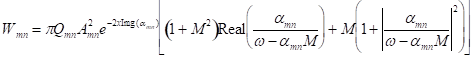 .
.
Since
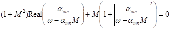 ,
,
we have
![]() .
(51)
.
(51)
A cutoff mode is also called evanescent wave. An evanescent wave transports no net acoustic energy (in stationary media), for pressure and axial velocity are 900 out of phase. There is an abrupt change of acoustic intensity from cut-on modes to cut-off modes (Pierce, p316). Physics meaning of evanescent waves (cut-off modes) in duct is: the waves decay very fast away from its source. But the medium is ideal and thus the decay is not due to viscous dissipation. Each fluid element oscillates with sound energy. This energy is established at the unsteady stage when there is transmitted energy across the duct section. After it gets to the steady stage, there is no net transmitted sound across duct section.
(m, n) Mode
in Both Axial Directions
 (52)
(52)
![]() .
.
For a cut-on mode,
![]() ,
, ![]() ,
,
![]() ,
,
 .
.
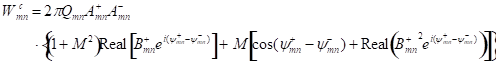
The cross term is zero:
![]()
Therefore,
![]() .
(53)
.
(53)
For a cut-off mode,
![]() ,
, ![]() ,
,
![]() ,
, ![]() ,
, ![]() .
.
![]() ,
,
Since
![]() ,
,
we have
![]() .
(54)
.
(54)
 ,
,
In Summary
(1)For each cut-on (m, n)
mode, if the wave propagates only
in one direction, ![]() ; if the wave
propagates in both directions,
; if the wave
propagates in both directions, ![]() ;
;
(2)For each cut-off (m, n)
mode, if the wave only ‘propagates’ in one direction, ![]() ; if the wave ‘propagates’ in both directions,
; if the wave ‘propagates’ in both directions, ![]() ;
;
(3)Total sound power is the sum of sound powers calculated from
each individual (m, n) mode.