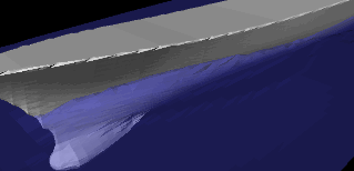
Bow of boat

Overhead view
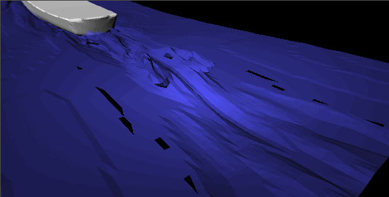
Stern of boat
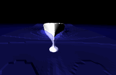
Front view
Boat-Wake Visualization using Open Inventor
Kevin Beason, Eric Hernandez, David Banks
April 26, 2000
Abstract
We wrote Open Inventor programs to create interactive visualizations of boat-wake data created by the theories of Dr. Sussman, a faculty member of the FSU Mathematics Department.
Introduction and Related Work
Dr. Sussman was a faculty member in the nearby FSU Mathematics Department with a program for simulating the wake left behind by a boat moving through the water. He could render a 3-D display of the boat and surface of the water but the image was static, in the sense that you could not rotate it and it didn’t move. Also the quality was pretty poor, but this was what was available to him using a program called "IDL".
He had a FORTRAN 90 program he wrote to generate the data1. On a 4 processor SGI with 4 gigabytes of memory his program could generate a time step every 4 minutes, but he had a dataset already generated from the 500th timeset. His data was a 128x96x96 grid containing a levelset function for the surface of the water and the velocity of the water, and some other information required for the simulation. The data was stored in a 170-megabyte text file.
We proposed to visualize the surface of the water and the velocity field of the moving water using the hardware-accelerated capabilities of the SGI computers available, using Open Inventor. This seemingly simple task was more than Dr. Sussman had done before, never having had a good view of his data but instead producing single, hard-to-see pictures.
Project Description
It took me a good 3 weeks just to have my program correctly read in his data from the 500th timestep. This was caused by many mistakes on my part. Luckily my professor, Dr. Banks, showed me a program called "Amira" that can quickly render an isosurface and I used this to take a quick-glance at Dr. Sussman’s data. This worked well and assured me that the data was correct. However, I needed my data in Inventor so I could do other, more interesting stuff with it.
After I could read the data, I figured out how to apply Dr. Banks implementation of the Marching Cubes algorithm, which worked well on one cube, to my entire grid of data. This was complicated because I didn’t really know how his program worked and I didn’t know Inventor well either.
This was the hardest part of the project. If I wasn’t doing marching cubes right, I was reading the data wrong. Also, things were drawn out because each run of the program required a 2-minute time overhead just to read in the massive 170-megabyte data file. Dr. Banks suggested I decimate the data, skipping every other value, to create a smaller, faster dataset. I followed his advice and created the data, which was about 8 times faster and cut down on debugging time by about a factor of 8.
I eventually got Marching Cubes to work after some more help from Dr. Banks. By now I could read in the air-water surface and rotate it in 3-D. The next step was to read in the boat surface and this was done easily. Soon I had the boat sitting in the water, and you could rotate it in 3-D.
Eric Hernandez put the finishing touches on this isosurface visualization. He added a large water surface beneath the boat, and tuned the water properties to give it a nice color and transparency. The transparency was a great help to the visualization, allowing viewers to see the hull beneath the surface of the water. This was another feature not present in prior visualizations by Dr. Sussman. Eric also rotated and translated the scene to have a good starting vantage, facing the front of the boat, when the program first displays.
The next step was to visualize the velocity vector field of the water beneath the boat. Had I enough time, I might have been able to get rid of all the bugs, but eventually I just gave up on this project altogether.
Instead of visualizing the water velocity, I created isosurfaces of the water at different timesteps in anticipation of creating an animation of the water flowing, per Dr. Banks suggestion.
I started from the beginning (timestep 0) using Dr. Sussman’s FORTRAN 90 code to generate successive timesteps and wrote each one out to disk for isosurface generation. The program ran over-night on a 4-processor SGI Onyx and only produced 10 steps. Worse, the water was almost still perfectly flat, even on the last (10th) step! This was one day before the presentation so something had to be done. Dr. Sussman showed me how to start the program using the 500th timestep datafile that he provided, and only write out every 10th timestep. By the following day we had 7 isosurfaces for timesteps 510-560.
Writing a program to display successive isosurfaces to form an animation was surprisingly easy. The only bad thing was that each isosurface was 14 megabytes and was real slow to read in. Each isosurface took one minute to read in, so it took 7 minutes to read in this simple 7-frame animation. The program ran the animation at 1 frame per second.
Results
In the end I had a scene file that I could view with "ivview". It was a scene graph of the water surface with the ship in it, at timestep 500, with nice colors and transparency on the water. The scene had about 50-100 thousand triangles and rendered at about 10 fps on the Onyx.
Better than this, I had an animation of the water surface that was 7 frames long, each frame constituting 10 timesteps starting at timestep 500, running at 1 Hz and 1 fps on the Onyx (It was slow). You can see a wave breaking behind the boat.
Figures

Bow of boat

Overhead view

Stern of boat

Front view
Footnotes:
1. Doug Dommermuth from SAIC helped write the code for modeling the ship flows (he helped with the multigrid solver).