Basic Homotopy
Contents
- Path space
- Type families as fibrations
- Homotopies and equivalences
- Theorems about weak equivalences
- Topological interlude
- Voevodsky’s definition of weak equivalence
- Half adjoint equivalences
- Properties of weak equivalences
We collect several Homotopy Theory-inspired constructions: homotopy equivalences, weak equivalences, homotopy fibers. We also give more type-theoretic constructions that are inspired by them: for instance, since sum types are total spaces of fibrations, we not only have the transport operation, but we can define several variants of the path-litfing operations that are available in Topology.
{-# OPTIONS --without-K --safe #-}

module basichomotopy where

open import mltt
open import negation using ( _⟺_ )
Let us also open a few submodules with lemmas from MLTT for recurrent usage:
open ≡-Reasoning
open ◾-lemmas
open ap-lemmas
open transport-lemmas
Path space
Following the homotopical interpretation of Martin-Löf Type Theory in a model category, Awodey-Warren, we interpret the identity type of a given type as a path space. Accordingly, we set the following definition:record Path {ℓ : Level} (A : Set ℓ) : Set ℓ where constructor path field p₀ : A p₁ : A ϖ : p₀ ≡ p₁ infixr 30 Path syntax Path A = A ᴵ syntax path p₀ p₁ ϖ = ϖ [ p₀ ↝ p₁ ]
We could have of course used a Sigma type in the definition. By opening the module, the names of the record’s fields become available in the global scope.
Type families as fibrations
One of the fundamental interpretations of HoTT is that type families, i.e. dependent types are interpreted as fibrations. In turn, the defining property of a fibration in a homotopy theory is the lifting one with respect to certain class of maps, in particular paths.
Therefore we prove that this is the case in our minimal type theory: we show, mostly following the HoTT book, that a dependent type P : A → Set ℓ' then it has such a notion of path lifting. There are several versions of this that we can define.
-- naive version of pathlift
pathlift : ∀{ℓ ℓ'} {A : Set ℓ} {P : A → Set ℓ'} {x y : A} {u : P x} (p : x ≡ y) →
           x , u ≡ y , (transport P p u)
pathlift {ℓ} {ℓ'} {A} {P} {x} {.x} {u} refl = idp (x , u)

-- this shows that pathlift projects back to the identity of x ≡ y
pathlift-covers-path : ∀{ℓ ℓ'} {A : Set ℓ} {P : A → Set ℓ'} {x y : A} {u : P x} (p : x ≡ y) →
                       ap π₁ (pathlift {P = P} {u = u} p) ≡ p
pathlift-covers-path {ℓ} {ℓ'} {A} {P} {x} {.x} {u} refl = refl
Given a (dependent) function f : Π[ x ∈ A] P x (the section of a fibration), we can re-interpret it as a global function f : A → Σ[ x ∈ A ] P x, that is, a section of the projection from the total space Σ A P to the base A of the fibration defined by f. This has already been done with
Γ : ∀ {ℓ ℓ'} {A : Set ℓ} {P : B → Set ℓ'} → Π A P → (A → Σ A P)global = ΓNow, if
f : Π A P, applying Γ f to an identification p : x ≡ y in the base gives a path in the total space, so one can consider ap (Γ f) p as a lift to the total space.
apd-naive : ∀ {ℓ ℓ'} {A : Set ℓ} {P : A → Set ℓ'} {x y : A} (f : Π[ x ∈ A ] P x) →
            x ≡ y → (global f) x ≡ (global f) y
apd-naive f p = ap (global f) p
which of course maps down to the base to a path (propositionally) equal to
p, that is, apd-naive is a form of pathlift:
apd-naive-pathlift : ∀ {ℓ ℓ'} {A : Set ℓ} {P : A → Set ℓ'} {x y : A} {p : x ≡ y}
                     (f : Π[ x ∈ A ] P x) → ap π₁ (apd-naive f p) ≡ p
apd-naive-pathlift {p = p} f = ap π₁ (apd-naive f p) ≡⟨  (ap∘ (global f) π₁ p) ⁻¹ ⟩
                               ap (π₁ ∘′ (global f)) p ≡⟨  apid p ⟩
                               p ∎
However, the commonly found form of dependent ap, or apd, is as follows:
apd : ∀ {ℓ ℓ'} {A : Set ℓ} {P : A → Set ℓ'} (f : Π[ x ∈ A ] P x) {x y : A} →
      (p : x ≡ y) → transport P p (f x) ≡ f y
apd f {x} refl = idp (f x)
So its type is altogether different. Given a dependent function, what apd does is to map an identification p : x ≡ y in the base to an identification in the fiber over the terminal point between the transport of f x and f y.
There are several variants of this concept, as well as several complementary notions that altogether provide: (1) a better understanding of the identity type in (the total space of) a fibration; and (2) an identity principle for them. We use some concepts from the UniMath library, originally due to Voevodsky.
First, we define the “total space” corresponding to the dependentapd: more precisely, if P : A → Set ℓ' is a dependent type, which we view as a fibration, then PathPair below constructs the fibration whose base consists of identifications, i.e. paths, in A and whose fibers consists of vertical identity types in the fibers of the terminal points:
PathPair : ∀ {ℓ ℓ'} {A : Set ℓ} {P : A → Set ℓ'} (u v : Σ A P) → Set (ℓ ⊔ ℓ')
PathPair {P = P} u v = Σ[ p ∈ (π₁ u ≡ π₁ v) ] ( transport P p (π₂ u) ≡ (π₂ v) )

infix 30 PathPair
syntax PathPair u v = u ╝ v
According to this definition,
PathPair can be pictured as the total space of a fibration. (Exercise: which one?) Then the dependent apd appears as a section:
apd-is-section : ∀ {ℓ ℓ'} {A : Set ℓ} {P : A → Set ℓ'} (f : Π[ x ∈ A ] P x) {x y : A} →
                 x ≡ y → (x , f x) ╝ (y , f y)
apd-is-section f = global (apd f)
Since
PathPair provides a decomposition of the paths in the Sigma type associated to a dependent type, there should be a relation with the type of paths (without condition). This is obtained in the following lemmas.
PathPair→PathΣ : ∀ {ℓ ℓ'} {A : Set ℓ} {P : A → Set ℓ'} {u v : Σ A P} →
                 u ╝ v → u ≡ v
PathPair→PathΣ {u = x , s} {v = .x , t} (refl , q) = ap (λ _ → x , _) q

PathΣ→PathPair : ∀ {ℓ ℓ'} {A : Set ℓ} {P : A → Set ℓ'} {u v : Σ A P} →
                 u ≡ v → u ╝ v
PathΣ→PathPair {u = u} {v = v} q = (ap π₁ q) , pathinfiber q
                                   where
                                     pathinfiber : ∀ {ℓ ℓ'} {A : Set ℓ} {P : A → Set ℓ'} {u v : Σ A P}
                                                   (q : u ≡ v) → transport P (ap π₁ q) (π₂ u) ≡ π₂ v
                                     pathinfiber {u = u} refl = idp (π₂ u)
The two functions
PathPair→PathΣ and PathΣ→PathPair are enough to establish the logical equivalence between u ≡ v and u ╝ v
module _ {ℓ ℓ' : Level} {A : Set ℓ} {P : A → Set ℓ'} where

  PathPair⇔PathΣ : {u v : Σ A P} → (u ╝ v) ⟺ (u ≡ v)
  Σ.fst (PathPair⇔PathΣ ) = PathPair→PathΣ
  Σ.snd (PathPair⇔PathΣ ) = PathΣ→PathPair
But in fact we can do better and prove that these functions are quasi-inverses. When we have the notion of weak or homotopy equivalence in place we will be able to prove that the types
u ≡ v and u ╝ v are equivalent. For the time being let us prove the following:
PathΣ-equiv : ∀ {ℓ ℓ'} {A : Set ℓ} {P : A → Set ℓ'} {u v : Σ A P} {q : u ≡ v} →
                PathPair→PathΣ (PathΣ→PathPair q) ≡ q
PathΣ-equiv {q = refl} = idp (refl)

PathPair-Equiv : ∀ {ℓ ℓ'} {A : Set ℓ} {P : A → Set ℓ'} {u v : Σ A P} {q : u ╝ v} →
                PathΣ→PathPair (PathPair→PathΣ q) ≡ q
PathPair-Equiv {u = u} {.(Σ.fst u) , .(Σ.snd u)} {q = refl , refl} = refl
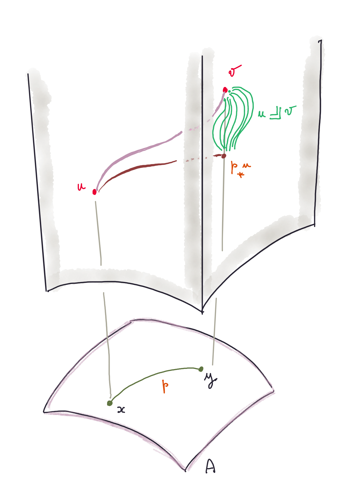
In the figure to the left, we have a schematic depiction of the situation so far. The type A, the base, is at the bottom, and on top we have the total space of the fibration, namely the type Σ A P. Given a path p : x ≡ y in the base, and two points u and v in the fibers lying over the initial and terminal points of the path in the base.
A simple path lift would be a path q : Σ A P in the total space without additional conditions.
The transport transport P p u is denoted \(p_*u\) in the figure. The type u ╝ v consists of the paths in the fiber between transport P p u and v.
The theorems we are proving essentially provide a decomposition of the type of paths u ≡ v into a path from u to its transport transport P p u and then a path in the fiber over y = π₁ x. Note, however, that these paths in the fiber fully “depend” on p : x ≡ y, so it is slightly incorrect to picture them as we did here.
Although not used until much later, it is convenient to have a separate name for the dependent type underlying the ╝ construction. This construction, which we call PathFiber, implements the notation \(p_*\) for the transport operation. We implement it via a syntax declaration.
PathFiber : ∀ {ℓ ℓ'} {A : Set ℓ} {P : A → Set ℓ'} {x y : A} (p : x ≡ y) (s : P x) (t : P y) → Set ℓ'
PathFiber {P = P} p s t = transport P p s ≡ t

infix 30 PathFiber
syntax PathFiber p s t =  p ✴ s ≡ t
The final piece of type-theoretic construction that we want to mention is PathOver, defined, among other places, in the foundation part of the UniMath library. To a path
p : x ≡ y and terms s : P x and t : P y we assign the type of paths from u to v lying over p.
PathOver : ∀ {ℓ ℓ'} {A : Set ℓ} (P : A → Set ℓ') {x y : A} (p : x ≡ y) (s : P x) (t : P y) → Set ℓ'
PathOver P refl s t = s ≡ t

infix 30 PathOver
syntax PathOver P p s t = s ≡[ P ↓ p ] t
The relation between PathOver and PathPair is the following
PathOver→PathPair : ∀ {ℓ ℓ'} {A : Set ℓ} {P : A → Set ℓ'} {x y : A} (p : x ≡ y) (s : P x) (t : P y) →
                    s ≡[ P ↓ p ] t → (x , s) ╝ (y , t)
PathOver→PathPair {P = P} refl s t q = refl , q

PathPair→PathOver : ∀ {ℓ ℓ'} {A : Set ℓ} {P : A → Set ℓ'} {u v : Σ A P }
                    (q : u ╝ v) → (π₂ u) ≡[ P ↓ (π₁ q) ] (π₂ v)
PathPair→PathOver (refl , q~) = q~

PathOver→PathΣ : ∀ {ℓ ℓ'} {A : Set ℓ} {P : A → Set ℓ'} {x y : A} (p : x ≡ y) (s : P x) (t : P y) →
                     s ≡[ P ↓ p ] t → (x , s) ≡ (y , t)
PathOver→PathΣ {P = P} p s t = PathPair→PathΣ ∘′ (PathOver→PathPair p s t)

PathΣ→PathOver : ∀ {ℓ ℓ'} {A : Set ℓ} {P : A → Set ℓ'} {u v : Σ A P} (q : u ≡ v) → (π₂ u) ≡[ P ↓ (ap π₁ q) ] (π₂ v)
PathΣ→PathOver q = PathPair→PathOver ( (PathΣ→PathPair q) )
Homotopies and equivalences
We turn to the definition of homotopy between (dependent) functions and to the definition of both weak equivalence and homotopy equivalence. Several of definitions are possible, and we will try to analyze the issue in some detail.
Function homotopy
First we define the notion of homotopy between two (possibly dependent) functions terms. Let us take advantage of the Π-notation we have introduced in the basic Martin-Löf Type Theory module.infix 3 _~_ _~_ : ∀ {ℓ ℓ'} {A : Set ℓ}{P : A → Set ℓ'} (f g : Π[ x ∈ A ] P x) → Set (ℓ ⊔ ℓ') _~_ {ℓ} {ℓ'} {A} {P} f g = Π[ x ∈ A ] ((f x) ≡ (g x))
The definition is in fact a universal quantifier: this definition states that to each term x : A we assign the type of paths, i.e. indentifications, from f(x) to g(x). Therefore, a term of the form
h : f ~ gwill provide, for each term x : A, an identification h x : f x ≡ g x.
Note that the definition we gave is “by value:” the path provided by the homotopy depends on the term x : A. This is different from the other possible notion of “homotopy” between two function types, namely to simply define it as an identification of the form h : f ≡ g. These two notions only become the same if (the axiom of) Function Extensionality is assumed. The latter is also a consequence of Univalence.
module ~-lemmas {ℓ ℓ' : Level} {A : Set ℓ}  where

  private
    variable
      P : A → Set ℓ'

  -- Reflexive
  ~-refl : {f : Π[ x ∈ A ] P x} → (f ~ f)
  ~-refl  = λ x → refl


  -- Symmetric
  ~-sym : {f g : Π[ x ∈ A ] P x} → (f ~ g) → (g ~ f)
  ~-sym p = λ x → (p x) ⁻¹

  syntax ~-sym p = p ~⁻¹


  -- Transitive
  ~-trans : {f g h : Π[ x ∈ A ] P x} → (f ~ g) → (g ~ h) → (f ~ h)
  ~-trans p q = λ x → (p x) ◾ (q x)

  syntax ~-trans p q = p ~◾~ q


  -- Precomposition
  ~-comp : ∀ {i} {X : Set i} {f g : Π[ x ∈ A ] P x} → f ~ g → (h : X → A) →
            (f ∘ h) ~ (g ∘ h)
  ~-comp p h = λ x → p (h x)

  syntax ~-comp p h = p ~∘ h
Note that if we want to post-compose a homotopy with a dependent function, such as the one below, we can not simply use
h ∘ f ~ h ∘ g, because h (f x) : C (f x), whereas h (g x) : C (g x), so the types are different. We need to transport the term h (f x) to C (g x), which is accomplished by the following item:
  -- Postcomposition
  apd-~ : ∀ {ℓ''} {C : {x : A} → P x → Set ℓ''}
          (h : {x : A} (y : P x) → C y) {f g : Π[ x ∈ A ] P x} →
          (p : f ~ g) →
          (λ (x : A) → (transport (λ (y : P x) → C {x} y) (p x)) ((h ∘ f) x) ) ~ (h ∘ g)
  apd-~ h p = λ x → apd h (p x)
It is convenient to have a non-dependent version of the post-composition of a homotopy with a function:
  -- Non-dependent composition
  ap-~ : ∀ {ℓ''} {B : Set ℓ'} {C : Set ℓ''} (h : B → C) {f g : A → B} →
         (p : f ~ g) → (h ∘′ f) ~ (h ∘′ g)
  ap-~ h p = λ x → ap h (p x)

  syntax ap-~ h p = h ∘~ p
Homotopy equivalences
In Topology we say that a map \(f \colon X → Y\) is a homotopy equivalence if there exists a \(g \colon Y → X\) such that \(f ∘ g ∼ \mathrm{id}_Y\) and \(g ∘ f ∼ \mathrm{id}_X\). We say that \(g\) is a quasi-inverse to \(f\). We implement this notion by defining the type of quasi-inverses of f : A → B
qinv : ∀ {ℓ ℓ'} {A : Set ℓ} {B : Set ℓ'} (f : A → B) → Set (ℓ ⊔ ℓ')
qinv f = Σ[ g ∈ (codomain f → domain f) ] ((f ∘′ g ~ id) × (g ∘′ f ~ id))
We read this type to state that there exists a g : B → A such that g ∘ f ~ id and f ∘ g ~ id. Therefore, a term
qif : qinv fcorresponds to a proof that our function possesses a quasi-inverse.
Given two types, we can also introduce the type of homotopy equivalences between the two:_≅_ : ∀ {ℓ ℓ'} (A : Set ℓ) (B : Set ℓ') → Set (ℓ ⊔ ℓ') A ≅ B = Σ[ f ∈ (A → B) ] (qinv f)
A term of this type would be something of the form (f , (g , (ε , η))), where f : A → B, and g : B → A is a quasi-inverse, with a proof of the two required homotopy conditions.
Exercise: Given a dependent type P : A → Set ℓ, and terms u v : Σ A P, prove that (u ≡ v) ≅ (u ╝ v). What is the appropriate statement if you use PathOver?
Weak equivalences
There exists of course a different notion of what it means to be equivalent. In the standard case, that is in the category \(\mathbf{Top}\), we say that \(f \colon X → Y\) is a weak equivalence if it induces an isomorphism between all homotopy groups. In general, such an \(f\) need not be quasi-invertible. However, a weak equivalence is a homotopy equivalences if its domain and codomain are cofibrant-fibrant. A similar logical equivalence between the type of homotopy equivalences and the soon-to-be-defined one of weak equivalence is available in our type-theoretic environment.
Let us begin by giving the simplest definition of weak equivalence. This is almost the same as that of homotopy equivalence, except that we do not require the left and right inverses to be the same.iseq : ∀ {ℓ ℓ'} {A : Set ℓ} {B : Set ℓ'} (f : A → B) → Set (ℓ ⊔ ℓ') iseq f = ( Σ[ g ∈ (codomain f → domain f) ] ( (f ∘′ g) ~ id) ) × ( Σ[ h ∈ (codomain f → domain f) ] ( (h ∘′ f) ~ id) )Similarly, let us define the type of weak equivalences between two types:
infix 3 _≃_
_≃_ : ∀ {ℓ ℓ'} (A : Set ℓ) (B : Set ℓ') → Set (ℓ ⊔ ℓ')
A ≃ B = Σ[ f ∈ (A → B) ] (iseq f)
This time a term of this type would be of the form (f , (g , ε) , (h , η)), consisting of a function f : A → B, right and left inverses (g , ε) and (h , η) together with proofs of these statements.
Weak vs. homotopy equivalences
We prove that the types A ≅ B and A ≃ B are in fact logically equivalent. The statement expressing this fact is
∀ {ℓ ℓ'} {A : Set ℓ} {B : Set ℓ'} → (A ≃ B) ⟺ (A ≅ B)but in fact we will have some use for the actual components of the proof. Therefore we proceed by building explicit functions back and forth between these two types.
First, we prove the relatively obvious fact that iff : A → B is a homotopy equivalence, then it must be a weak equivalence.
qinv→iseq : ∀ {ℓ ℓ'} {A : Set ℓ} {B : Set ℓ'} (f : A → B) → qinv f → iseq f
Σ.fst (qinv→iseq f (g , (ε , η))) = g , ε
Σ.snd (qinv→iseq f (g , (ε , η))) = g , η
The converse direction is more difficult, and it presents us with a dilemma: in producing a quasi-inverse to f : A → B we must choose one of the two partial quasi-inverses that are part of the data of a weak equivalence. This will create an undesirable asymmetry in the proof of the statement. Better versions of the notion of weak equivalence circumvent this particular problem. For now, let us go ahead and produce a proof by choosing a specific quasi-inverse.
iseq→qinv : ∀ {ℓ ℓ'} {A : Set ℓ} {B : Set ℓ'} (f : A → B) → iseq f → qinv f
Σ.fst (iseq→qinv f ((g , ε) , (h , η))) = g
Σ.fst (Σ.snd (iseq→qinv f ((g , ε) , (h , η)))) = ε
Σ.snd (Σ.snd (iseq→qinv f ((g , ε) , (h , η)))) = (δ ~∘ f) ~◾~ η
  where
    open ~-lemmas
    δ : g ~ h
    δ = ((η ~∘ g) ~⁻¹) ~◾~ ( h ∘~ ε )
In short, we construct a homotopy from the right inverse of \(f\) to the left one. Clearly we could have used the mirror argument and decided upon the left inverse to be our choice.
Armed with these two proposition, we can prove the types of homotopy equivalences and weak equivalences are logically equivalent:weq-is-hoeq : ∀ {ℓ ℓ'} {A : Set ℓ} {B : Set ℓ'} → (A ≃ B) ⟺ (A ≅ B) Σ.fst weq-is-hoeq (f , iseqf) = f , iseq→qinv f iseqf Σ.snd weq-is-hoeq (f , qif) = f , qinv→iseq f qif
Theorems about weak equivalences
Let us look at the usual relations for the notion of weak equivalence. As usual, we put them in a module
module ≃-lemmas where

  open ~-lemmas

  -- Reflexive
  ≃-refl : ∀ {ℓ} {A : Set ℓ} → A ≃ A
  Σ.fst ≃-refl = id
  Σ.fst (Σ.snd ≃-refl) = id , (λ _ → refl)
  Σ.snd (Σ.snd ≃-refl) = id , (λ _ → refl)
To prove the symmetry we take advantage of
iseq→qinv to turn a weak equivalence into a homotopy one. Then we can simply swap the proofs and convert it back to a weak equivalence. Like in other cases, the symmetry property translate to the fact that weak equivalences, as well as, homotopies, can be inverted.
  -- Symmetry
  ≃-sym : ∀ {ℓ ℓ'} {A : Set ℓ} {B : Set ℓ'} → A ≃ B → B ≃ A
  ≃-sym (f , iseqf) = let f⁻¹ , qif = iseq→qinv f iseqf
                      in f⁻¹ , qinv→iseq f⁻¹ (f , (×-swap qif))
Transitivity is just the composition of weak equivalences. The composition at the level of functions is the first component of the resulting type. We must also provide proofs, i.e. function homotopies, that provide the correct left and right inverses to the compositinon.
  -- Transitivity
  ≃-trans : ∀ {ℓ ℓ' ℓ''} {A : Set ℓ} {B : Set ℓ'} {C : Set ℓ''} →
            A ≃ B → B ≃ C → A ≃ C
  Σ.fst (≃-trans (f , iseqf) (g , iseqg)) = g ∘′ f
  Σ.fst (Σ.snd (≃-trans (f , iseqf) (g , iseqg))) = let r , ε = π₁ iseqf
                                                        v , τ = π₁ iseqg
                                                    in (r ∘′ v) , (( g ∘~ (ε ~∘ v)) ~◾~ τ)
  Σ.snd (Σ.snd (≃-trans (f , iseqf) (g , iseqg))) = let l , η = π₂ iseqf
                                                        u , σ = π₂ iseqg
                                                    in (l ∘′ u) , ((l ∘~ (σ ~∘ f)) ~◾~ η)

  -- Syntax declarations
  ≃id = ≃-refl
  syntax ≃-sym f = f ≃⁻¹
  syntax ≃-trans f g = f ≃◾≃ g
Since the situation is formally analogous to that of propositional equality, we can provide a similar reasoning module:
module ≃-Reasoning where

  open ≃-lemmas

  infix 3 _≃∎
  infixr 2 _≃⟨_⟩_

  _≃⟨_⟩_ : ∀ {ℓ ℓ' ℓ''} (A : Set ℓ) {B : Set ℓ'} {C : Set ℓ''} → A ≃ B → B ≃ C → A ≃ C
  A ≃⟨ e ⟩ f = e ≃◾≃ f

  _≃∎ : ∀ {ℓ} (A : Set ℓ) → A ≃ A
  A ≃∎ = ≃id {A = A}
An important example of weak equivalence is the map provided by the transport operation in a dependent type:
transport-is-≃ : ∀ {ℓ ℓ'} {A : Set ℓ} (P : A → Set ℓ') {x y : A} (p : x ≡ y) → iseq (transport P p)
transport-is-≃ P {x} refl = π₂ ( ≃-lemmas.≃id {A = P x} )

transport→≃ : ∀ {ℓ ℓ'} {A : Set ℓ} (P : A → Set ℓ') {x y : A} (p : x ≡ y) → P x ≃ P y
transport→≃ P p = (transport P p) , transport-is-≃ P p
Finally, we have that if f is homotopic to g, and g is a weak equivalence, then so is f:
homot-to-we-is-we : ∀ {ℓ ℓ'} {A : Set ℓ} {B : Set ℓ'} {f g : A → B} →
                    (f ~ g) → iseq g → iseq f
Σ.fst (Σ.fst (homot-to-we-is-we φ ((h , _) , _ , _))) = h
Σ.snd (Σ.fst (homot-to-we-is-we φ ((h , ε) , _ , _))) = λ b → φ (h b) ◾ (ε b)
Σ.fst (Σ.snd (homot-to-we-is-we φ ((_ , _) , k , _))) = k
Σ.snd (Σ.snd (homot-to-we-is-we φ ((_ , _) , k , η))) = λ b → (ap k (φ b)) ◾ (η b)
Topological interlude
Higher homotopies
Let us define the type of homotopies of homotopies. Therefore for two dependent functionsf g : (x : A) → P x and two homotopies ε and η between them, we define the type of identifications (x : A) → (ε x) ≡ (η x). Leaving most variables implicit, the definition is not too different from the function homotopy defined above.
infix 3 _≈_
_≈_ : ∀ {ℓ ℓ'} {A : Set ℓ}{P : A → Set ℓ'}
      {f g : Π[ x ∈ A ] P x} (ε η : f ~ g) → Set (ℓ ⊔ ℓ')
_≈_ {A = A} ε η = Π[ x ∈ A ] (ε x ≡ η x)
Contractibility and connectedness
In analogy with spaces, we say that a type is contractible if there exists a term, the center, and for each term an identification of it with the center. The corresponding proposition that a type is contractible asserts the existence of the contraction center as follows:iscontr : ∀ {ℓ} (A : Set ℓ) → Set ℓ iscontr A = Σ[ c ∈ A ] ( Π[ a ∈ A ] (c ≡ a) ) iscontr-center : ∀ {ℓ} (A : Set ℓ) → iscontr A → A iscontr-center A (c , p) = c iscontr-path-center : ∀ {ℓ} (A : Set ℓ) (is : iscontr A) (a : A) → (iscontr-center A is) ≡ a iscontr-path-center A (c , γ) a = γ aFor example, 𝟙 does have this property:
𝟙-iscontr : iscontr 𝟙
𝟙-iscontr =  * , (𝟙-induction (λ x → * ≡ x) refl)
Note that the goal to the proof is to provide (x : 𝟙) → * ≡ x, which is achieved by induction.
contr-is-we-to-𝟙 : ∀ {ℓ} {A : Set ℓ} (A-contr : iscontr A) → 𝟙 ≃ A
contr-is-we-to-𝟙 {ℓ} {A} A-contr = (𝟙-to-contr A-contr) , ((!𝟙 , contr-𝟙-contr A-contr) , (!𝟙 , 𝟙-contr-𝟙 A-contr))
  where
    𝟙-to-contr : ∀ {ℓ} {A : Set ℓ} → iscontr A → 𝟙 → A
    𝟙-to-contr A-contr = λ _ → π₁ (A-contr)

    contr-𝟙-contr : ∀ {ℓ} {A : Set ℓ} (A-contr : iscontr A) → Π[ a ∈ A ] (((𝟙-to-contr A-contr) ( !𝟙  a) ) ≡ a )
    contr-𝟙-contr A-contr = λ x → π₂ (A-contr) x

    𝟙-contr-𝟙 : ∀ {ℓ} {A : Set ℓ} (A-contr : iscontr A) → Π[ t ∈ 𝟙 ] ( !𝟙 ( (𝟙-to-contr A-contr) t) ≡ t )
    𝟙-contr-𝟙 A-contr = π₂ (𝟙-iscontr)
In fact this is a logical equivalence:
is-we-to-𝟙-iscontr : ∀ {ℓ} {A : Set ℓ} → 𝟙 ≃ A → iscontr A
is-we-to-𝟙-iscontr {ℓ} {A} φ = center , contraction
  where
    u : 𝟙 → A
    u = π₁ φ

    v : A → 𝟙
    v = π₁ (π₁ (π₂ φ)) --right-inverse

    ε : u ∘′ v ~ id
    ε = π₂ (π₁ (π₂ φ))

    center : A
    center = u *

    contraction : ∀ a → center ≡ a
    contraction = λ a → ε a --because u (v a) = u * = center
So we have a logical equivalence:
iscontr-isequiv-𝟙 : ∀ {ℓ} {A : Set ℓ} → iscontr A ⟺ (𝟙 ≃ A)
iscontr-isequiv-𝟙 {A} = contr-is-we-to-𝟙 , is-we-to-𝟙-iscontr
It immediately follows that for two weakly equivalent types one is contractible if and only if the other is. And since being weakly equivalent is a symmetric condition, we can just prove:
we-and-contr-implies-contr : ∀ {ℓ ℓ'} {A : Set ℓ} {B : Set ℓ'} →
                             A ≃ B → iscontr A → iscontr B
we-and-contr-implies-contr {A = A} {B} φ isca = iscb
   where
     u : 𝟙 ≃ A
     u = contr-is-we-to-𝟙 isca

     v : 𝟙 ≃ B
     v = 𝟙 ≃⟨ u ⟩
         A ≃⟨ φ ⟩
         B ≃∎
       where
         open ≃-Reasoning

     iscb : iscontr B
     iscb = is-we-to-𝟙-iscontr v
Clearly, in the other direction, two contractible types are weakly equivalent, because they are both equivalent to 𝟙:
two-contractibles-are-we : ∀ {ℓ ℓ'} {A : Set ℓ} {B : Set ℓ'} →
                           iscontr A → iscontr B → A ≃ B
two-contractibles-are-we {A = A} {B} isca  iscb = φ
   where
     u : 𝟙 ≃ A
     u = contr-is-we-to-𝟙 isca

     v : 𝟙 ≃ B
     v = contr-is-we-to-𝟙 iscb

     φ : A ≃ B
     φ = A ≃⟨ u ≃⁻¹ ⟩
         𝟙 ≃⟨ v  ⟩
         B ≃∎
       where
         open ≃-lemmas
         open ≃-Reasoning
Another concept we can transport into type theory is that of a type being path connected. We say that for any two terms of that type there is an identification between them. Here is the corresponding proposition.
ispathconn : ∀ {ℓ} (A : Set ℓ) → Set ℓ
ispathconn A = (x y : A) → x ≡ y
Of course, a contractible type must be path connected:
contr-is-pathconn : ∀ {ℓ} (A : Set ℓ) → iscontr A → ispathconn A
contr-is-pathconn A (c , γ) x y = x ≡⟨ (γ x) ⁻¹ ⟩
                                  c ≡⟨ γ y ⟩
                                  y ∎
Again, we have some obvious examples: 𝟘 and 𝟙.
𝟘-ispathconn : ispathconn 𝟘
𝟘-ispathconn x y = !𝟘 {B = (x ≡ y)} x

𝟙-ispathconn : ispathconn 𝟙
𝟙-ispathconn = contr-is-pathconn 𝟙 (𝟙-iscontr)
Returning to the fact that maps of contractible types are weak equivalences, it is more advantageous to have some degree of control on the map itself, so we prove what essentially is the same statement in a more explicit way: this uses the property of being path-connected.
map-of-contractibles-is-we : ∀ {ℓ ℓ'} {A : Set ℓ} {B : Set ℓ'} →
                             (f : A → B) → iscontr A → iscontr B → iseq f
map-of-contractibles-is-we f isa isb = qinv→iseq f (g , ε , η)
  where
    A = domain f
    B = codomain f

    g : B → A
    g b = iscontr-center A isa

    ε : f ∘′ g ~ id
    ε b =  contr-is-pathconn B isb (f (g b)) b

    η : g ∘′ f ~ id
    η = iscontr-path-center A isa
Retractions
Retractions are familiar from Topology. We say that \(A\) is a retraction of \(B\) if there is a map \(r \colon B → A\) that has a section, i.e. a map \(s \colon A → B\) which is a right-inverse: \(r ∘ s = id\). The standard case is that of an inclusion \(i \colon A ⊂ B\) which is a section to \(r \colon B → A\), that is \(r ∘ i = id\).
Retractions can be used to transfer properties. We will adopt the same stance for types, with obvious modifications.
First, let us state that a functionr : B → A has a section:
has-sect : ∀ {ℓ ℓ'} {A : Set ℓ} {B : Set ℓ'} → (A → B) → Set (ℓ ⊔ ℓ')
has-sect r = Σ[ s ∈ (codomain r → domain r) ] (r ∘′ s ~ id)
This is just the type of possible sections of r : A → B, which might just be empty. A term of this type consists of a pair s , η of a function s : B → A with the datum of η : r ∘′ s ~ id. Thus this is data, not a property: it is possible to have another pair s , η' with the same underlying function, but with a different homotopy.
A is a retraction of the type B, in symbols A ◅ B if there is a function r : B → A which has a section:
_◅_ : ∀ {ℓ ℓ'} → Set ℓ → Set ℓ' → Set (ℓ ⊔ ℓ')
A ◅ B = Σ[ r ∈ (B → A) ] (has-sect r)
We can extract the components of a term in a retraction type
retract : ∀ {ℓ ℓ'} {A : Set ℓ} {B : Set ℓ'} → (A ◅ B) → (B → A)
retract (r , (s , η)) = r

sect : ∀ {ℓ ℓ'} {A : Set ℓ} {B : Set ℓ'} → (A ◅ B) → (A → B)
sect (r , (s , η)) = s

retract-homotopy : ∀ {ℓ ℓ'} {A : Set ℓ} {B : Set ℓ'} → (ρ : A ◅ B) →
                   (retract ρ) ∘′ (sect ρ) ~ id
retract-homotopy (r , (s , η)) = η

retract-has-sect : ∀ {ℓ ℓ'} {A : Set ℓ} {B : Set ℓ'} → (ρ : A ◅ B) →
                   has-sect (retract ρ)
retract-has-sect (r , σ) = σ
The identity map is a retraction:
◅-id : ∀ {ℓ} → (A : Set ℓ) → (A ◅ A)
◅-id A = id , (id , (λ x → refl))
Retractions can be composed:
_◅◾_ : ∀ {ℓ ℓ' ℓ''} {A : Set ℓ} {B : Set ℓ'} {C : Set ℓ''} →
       A ◅ B → B ◅ C → A ◅ C
(r , (s , η)) ◅◾ (r' , (s' , η')) = (r ∘′ r') , ((s' ∘′ s) , η'')
  where
    open ~-lemmas
    η'' : (λ x → r (r' (s' (s x)))) ~ id
    η'' = (r ∘~ (η' ~∘ s)) ~◾~ η
--      alternatively, explicit
--      η'' x = r (r' (s' (s x))) ≡⟨ ap r (η' (s x)) ⟩
--              r (s x) ≡⟨ η x ⟩
--              x ∎
Whenever we have transitivity with an identity object we can introduce an appropriate reasoning module:
module ◅-Reasoning where

  infix 3 _◅∎
  infixr 2 _◅⟨_⟩_

  _◅⟨_⟩_ : ∀ {ℓ ℓ' ℓ''} (A : Set ℓ) {B : Set ℓ'} {C : Set ℓ''} →
          A ◅ B → B ◅ C → A ◅ C
  A ◅⟨ ρ ⟩ σ = ρ ◅◾ σ

  _◅∎ : ∀ {ℓ} (A : Set ℓ) → A ◅ A
  A ◅∎ = ◅-id A
Retractions can be used to show that something is contractible, in the sense that the retraction of something contractible is itself contractible:
retract-of-contr-is-contr : ∀ {ℓ ℓ'} {A : Set ℓ} {B : Set ℓ'} → (A ◅ B) →
                       iscontr B → iscontr A
retract-of-contr-is-contr (r , (s , η)) (centb , φ) = (r centb) , λ a → γ a
  where
    open ~-lemmas
    γ = (r ∘~ (φ ~∘ s)) ~◾~ η
--    Direct definition
--    γ = λ a → r centb ≡⟨ ap r (φ (s a)) ⟩
--              r (s a) ≡⟨ η a ⟩
--              a ∎
Finally, a lemma about retracting total spaces whenever the map between bases has a section. Recall map-over-total defined in the basic Martin-Löf Type Theory module. If P : A → Set ν and r : B → A has a section, so that in effect \(A\) is a retraction of \(B\), then the total space Σ[ a ∈ A ] P a is a retraction of the pull-back Σ[ b ∈ B ] P (f b). This lemma will be very important in discussing Voevodsky’s weak equivalences below.
Σ-pullback-retract : ∀ {ℓ ℓ' ν} {A : Set ℓ} {B : Set ℓ'} {P : A → Set ν} (r : B → A) →
                     has-sect r → ( Σ[ a ∈ A ] P a ) ◅ ( Σ[ b ∈ B ] P (r b) )
Σ-pullback-retract {A = A} {B = B} {P = P} r (s , η) = ρ , (σ , Η) -- Greek upper-case Eta
  where
    ρ : Σ[ b ∈ B ] P (r b) → Σ[ a ∈ A ] P a
    ρ (b , v) = (r b) , v

    σ : Σ[ a ∈ A ] P a → Σ[ b ∈ B ] P (r b)
    σ (a , u) = (s a) , transport P ((η a) ⁻¹) u

    Η : (y : Σ[ a ∈ A ] P a) → ρ (σ y) ≡ y
    Η (a , u) = PathPair→PathΣ (pp (a , u))
      where
        open transport-lemmas
        pp : (y : Σ[ a ∈ A ] P a) → ρ (σ y) ╝ y
        Σ.fst (pp (a , u)) = η a
        Σ.snd (pp (a , u)) = transport P (η a) (transport P (η a ⁻¹) u) ≡⟨ transport◾ (η a ⁻¹) (η a) ⟩
                             transport P ((η a ⁻¹) ◾ (η a)) u ≡⟨ transport≡ (linv (η a)) ⟩
                             u ∎
Stars of points
Given a point \(a ∈ A\), its star consists of pairs \((x , γ)\), where \(x ∈ A\) and \(γ : a ↝ x\) is a path. The corresponding type is the following:star : ∀ {ℓ} {A : Set ℓ} → A → Set ℓ star {ℓ} {A} a = Σ[ x ∈ A ] (a ≡ x)So a term of the star of
a : A is a pair consisting of term x : A and a path γ : x ≡ a. There is a privileged term of the star of a : A consisting of the pair a , refl, and given any other term (x , γ) : star a there is a path to the center, ultimately showing that the star of a point is contractible:
star-center : ∀ {ℓ} {A : Set ℓ} (a : A) → star a
star-center a = a , (idp a)

star-path-center : ∀ {ℓ} {A : Set ℓ} (a : A) ( u : star a) → u ≡ (star-center a)
star-path-center a (.a , refl) = idp (a , refl)

star-iscontr : ∀ {ℓ} {A : Set ℓ} (a : A) → iscontr (star a)
star-iscontr a = (star-center a) , (λ u → (star-path-center a u) ⁻¹)
Voevodsky’s concept of h-level
This is a good place to introduce the concept of h-level. The h-level proposition is defined by induction on ℕ, or rather, by a type of integers ≥ -2. Curiously, we can define h-levels relative to a given universe level ℓ.
We first define the index type ℤ[≥-2]
module h-level {ℓ : Level} where

  data ℤ[≥-2] : Set where
    –2 : ℤ[≥-2]
    suc : ℤ[≥-2] → ℤ[≥-2]

  h-level : Set ℓ → ℤ[≥-2] → Set ℓ
  h-level A –2 = iscontr A
  h-level A (suc n) = (x y : A) → h-level (x ≡ y) n
Homotopy fibers
Definition. Let \(f \colon A → B\) be a morphism in \(\mathbf{Top}\). The homotopy fiber of \(f\) at a point \(b ∈ B\) is
\[ \mathrm{hfib}_b(f) = \bigl\{ (a , γ) ∈ A × B^I \mathbin{\vert} f (a ) = γ (0) , γ (1) = b\bigr\}. \]
This definition can be seen as the concatenation of two pullbacks:
\[ \begin{array}{ccl} B^I_b & \longrightarrow & * \\ \downarrow & & \downarrow \scriptstyle{b} \\ B^I & \longrightarrow & B \end{array} \]
and
\[ \begin{array}{ccc} \mathrm{hfib}_b(f) & \longrightarrow & B^I_b \\ \downarrow & & \downarrow \\ A & \xrightarrow{f} & B \end{array} \]
The homotopy fiber construction allows to replace any map with a fibration.
The definition in Agda mimics the direct topological definitionhfib : ∀ {ℓ ℓ'} {A : Set ℓ} {B : Set ℓ'} (f : A → B) (b : B) → Set (ℓ ⊔ ℓ') hfib f b = Σ[ a ∈ domain f ] ((f a) ≡ b) -- extracting the components hfib-pt : ∀ {ℓ ℓ'} {A : Set ℓ} {B : Set ℓ'} {f : A → B} {b : B} → hfib f b → A hfib-pt (a , p) = a hfib-path : ∀ {ℓ ℓ'} {A : Set ℓ} {B : Set ℓ'} {f : A → B} {b : B} → (u : hfib f b) → f (hfib-pt u) ≡ b hfib-path (a , p) = p
Exercise: Write a definition in terms of pullbacks as above.
Constructions on Fibrations
By fibrations here we mean dependent dependent types P : A → 𝓤. The total space is the Σ-type Σ A P projecting over A. We want to collect a few results concerning the geometry of fibrations and their total spaces.
Given two type families P,Q : A → 𝓤, we want to think of f : Π[ x ∈ A ] (P x → Q x) as a fiberwise map. We can define the type of such fiberwise maps:
Hom : ∀ {ℓ ℓ' ℓ''} {A : Set ℓ} → (A → Set ℓ') → (A → Set ℓ'') → Set (ℓ ⊔ ℓ' ⊔ ℓ'')
Hom P Q = (x : domain P) → P x → Q x
Note that we can let the families take values in different universes. These induce maps between total spaces:
Hom→total : ∀ {ℓ ℓ' ℓ''} {A : Set ℓ} {P : A → Set ℓ'} {Q : A → Set ℓ''} →
        (Hom P Q) → Σ A P → Σ A Q
Hom→total f (x , s) = x , f x s
Once we have the map between the total spaces, we have that its homotopy fibers are equivalent to the pointwise homotopy fibers in the family:
fiber-total-equiv-fiber-Hom : ∀ {ℓ ℓ' ℓ''} {A : Set ℓ} {P : A → Set ℓ'} {Q : A → Set ℓ''}
                             (φ : Hom P Q) (x : A) (t : Q x) →
                             hfib (Hom→total φ) (x , t) ≃ hfib (φ x) t

fiber-total-equiv-fiber-Hom {P = P} φ x t = f , qinv→iseq f qi
  where
    f : hfib (Hom→total φ) (x , t) → hfib (φ x) t
    f ((y , s) , γ) = transport P (ap π₁ γ) s , ((transport-cov {f = φ} (ap π₁ γ) {s} ) ⁻¹ ◾  (π₂ pp))
      where
        pp : (y , φ y s) ╝ (x , t)
        pp = PathΣ→PathPair γ

    g : hfib (φ x) t → hfib (Hom→total φ) (x , t)
    g (s , γ) = (x , s) , PathPair→PathΣ pp
      where
        pp : (x , φ x s) ╝ (x , t)
        pp = refl , γ

    ε : f ∘′ g ~ id
    ε (s , refl) = refl

    η : g ∘′ f ~ id
    η ((y , s) , refl) = refl

    qi : qinv f
    qi = g , (ε , η)
The previous lemma, in conjunction with Voevodsky’s notion of weak equivalence, see below, implies that the map of total spaces is a weak equivalenc if and only if it is a fiberwise weak equivalence. This means that each f x : P x → Q x is a weak equivalence:
fib-iseq : ∀ {ℓ ℓ' ℓ''} {A : Set ℓ} {P : A → Set ℓ'} {Q : A → Set ℓ''}
           (f : Hom P Q) → Set (ℓ ⊔ ℓ' ⊔ ℓ'')
fib-iseq  {A = A} f = (x : A) → iseq (f x)
We are able to prove this by using the notion of weak equivalence we have introduced above:
iseq-total→fib-iseq : ∀ {ℓ ℓ' ℓ''} {A : Set ℓ} {P : A → Set ℓ'} {Q : A → Set ℓ''}
                      (f : Hom P Q) → fib-iseq f → iseq (Hom→total f)
iseq-total→fib-iseq {A = A} {P} {Q} f is = (ψ , Ε) , (χ , Η)
  where
    φ : Σ A P → Σ A Q
    φ = Hom→total f

    g h : Hom Q P
    g = λ x → π₁ (π₁ (is x))
    h = λ x → π₁ (π₂ (is x))

    ε : (x : A) → (f x) ∘′ (g x) ~ id
    ε = λ x → π₂ (π₁ (is x))

    η : (x : A) → (h x) ∘′ (f x) ~ id
    η = λ x → π₂ (π₂ (is x))

    ψ χ : Σ A Q → Σ A P
    ψ = Hom→total g
    χ = Hom→total h

    Ε : φ ∘′ ψ ~ id
    Ε (x , t) = x , f x (g x t) ≡⟨  PathPair→PathΣ {P = Q} pp ⟩
                x , t ∎
      where
        pp : (x , f x (g x t)) ╝ (x , t)
        pp = refl , (ε x t)

    Η : χ ∘′ φ ~ id
    Η (x , s) = x , h x (f x s) ≡⟨ PathPair→PathΣ {P = P} pp ⟩
                x , s ∎
      where
        pp : (x , h x (f x s)) ╝ (x , s)
        pp = refl , (η x s)
However, for the converse direction, the proof using the current version of weak equivalence is cumbersome and technically involved. We can use the theorem on homotopy fibers to prove the following intermediate result. Later, using Voevodsky’s notion of weak equivalence (see below), we will be able to prove the full converse to the above result. For now, we prove that one map has contractible fibers if and only if the other has fiberwise contractible fibers. The proof uses that for weakly equivalent types contractiblity is a logical equivalence.
contr-fiber-total-iff-contr-fiber-Hom :
    ∀ {ℓ ℓ' ℓ''} {A : Set ℓ} {P : A → Set ℓ'} {Q : A → Set ℓ''} (f : Hom P Q) →
    ( (v : Σ A Q) → iscontr (hfib (Hom→total f) v) ) ⟺ ((x : A) (t : Q x) → iscontr (hfib (f x) t))

Σ.fst (contr-fiber-total-iff-contr-fiber-Hom {A = A} {P} {Q} f) is  x t =
  we-and-contr-implies-contr (φ (x , t)) (is (x , t))
    where
      φ : (v : Σ A Q) → hfib (Hom→total f) v ≃ hfib (f (π₁ v)) (π₂ v)
      φ v = fiber-total-equiv-fiber-Hom f (π₁ v) (π₂ v)

Σ.snd (contr-fiber-total-iff-contr-fiber-Hom {A = A} {P} {Q} f) is v =
  we-and-contr-implies-contr ((φ v) ≃⁻¹) (is (π₁ v) (π₂ v))
    where
      φ : (v : Σ A Q) → hfib (Hom→total f) v ≃ hfib (f (π₁ v)) (π₂ v)
      φ v = fiber-total-equiv-fiber-Hom f (π₁ v) (π₂ v)
      open ≃-lemmas
The following useful theorem expresses (one half of) a universal property linking products and Σ-types. We can consider it as a property of fibrations, so it’s here. To clarify its content, suppose \(P , Q \colon A → 𝓤\) are two dependent types. There is a morphism
\[ r \colon ∏_{x : A} (P(x) × Q(x)) \longrightarrow (∏_{x : A} P(x)) × (∏_{x : A} Q(x)) \]
defined by \(f \mapsto (π₁ ∘ f , π₂ ∘ f)\). There is a morphism \(s\) in the other direction defined by \((g, h) \mapsto λx.(g(x), h(x))\). We prove below that \(r\) is a retraction, or, in other words, that the right hand side is a rectraction of the left. We actually do it for the more general case of dependent products instead of Cartesian products.
ΣΠ-univ : ∀ {ℓ ℓ' ℓ''} {A : Set ℓ} {P : (x : A) → Set ℓ'} {Q : (x : A) (u : P x) → Set ℓ''} →
          (Σ[ g ∈ (Π A P) ] (Π[ x ∈ A ] (Q x (g x))))  ◅ (Π[ x ∈ A ] ( Σ[ u ∈ P x ] (Q x u) ))
ΣΠ-univ {A = A} {P} {Q} = r , s , (λ { (g , h) → refl})
  where
    r : Π A (λ x → Σ (P x) (Q x)) → Σ (Π A P) (λ g → Π A (λ x → Q x (g x)))
    r f = (λ x → π₁ (f x)) , (λ x → π₂ (f x))

    s : Σ (Π A P) (λ g → Π A (λ x → Q x (g x))) → Π A (λ x → Σ (P x) (Q x))
    s (g , h) = λ x → (g x) , (h x)
If function extensionality is assumed, then the two types in the above statement are actually equivalent, because then one can prove the retraction in the other direction.
Naturality constructions
We collect some constructions inspired by 2-Category theory. The general idea, as expounded in the HoTT book, is that if functions between types behave as functors with respect to paths, via the applicative ap, then homotopies between functions behave as natural transformations.
Furthermore, if we interpret identifications as arrows, then higher identity types, in particular identifications of identifications, aquire operations, such as “horizontal composition,” whiskering, etc. that are reminiscent of the algebra of 2-Category theory.
Let us adopt the terms 1-cell and 2-cell to denote, respectively, an identification like p : x ≡ y and like α : p ≡ q.
Let us put these constructions in a module for future re-use.
module naturality where

  open import twocatconstructions public
Homotopy is a natural transformation (the second version is just for convenience, to avoid too many inverses)
  homot-natural : ∀ {ℓ ℓ'} {A : Set ℓ} {B : Set ℓ'} {f g : A → B} (h : f ~ g) {x y : A} (p : x ≡ y) →
                  (h x) ◾ (ap g p) ≡ (ap f p) ◾ (h y)
  homot-natural h {x} {.x} refl = ru (h x)

  homot-natural' : ∀ {ℓ ℓ'} {A : Set ℓ} {B : Set ℓ'} {f g : A → B} (h : f ~ g) {x y : A} (p : x ≡ y) →
                   (ap f p) ◾ (h y) ≡ (h x) ◾ (ap g p)
  homot-natural' h {x} {.x} refl = (ru (h x)) ⁻¹
and there is a type dependent version too:
  homNatD : ∀ {ℓ ℓ'} {A : Set ℓ} {P : A → Set ℓ'} {f g : Π A P} (h : f ~ g) {x y : A} (p : x ≡ y) →
            ap (transport P p) (h x) ◾ (apd g p) ≡ (apd f p) ◾ (h y)
  homNatD h {x} {.x} refl = ap id (h x) ◾ refl ≡⟨ ru (ap id (h x)) ⟩
                            ap id (h x) ≡⟨ apid (h x) ⟩
                            h x ∎
The following corollary expresses the naturality of a homotopy h : f ~ id. In the proof below we use homot-natural h (h x) .
  corollary[homot-natural] : ∀ {ℓ} {A : Set ℓ} {f : A → A} (h : f ~ id) {x : A} → (h (f x)) ≡ (ap f (h x))
  corollary[homot-natural]  {f = f} h {x} = h (f x) ≡⟨ (ru _ ) ⁻¹ ⟩
                                            h (f x) ◾ (idp (f x))            ≡⟨ first ⁻¹ ⟩
                                            h (f x) ◾ ((h x) ◾ (h x) ⁻¹)     ≡⟨ second ⁻¹ ⟩
                                            (h (f x) ◾ (h x)) ◾ (h x) ⁻¹     ≡⟨ third ⟩
                                            (h (f x) ◾ ap id (h x)) ◾ h x ⁻¹ ≡⟨ fourth ⟩
                                            (ap f (h x) ◾ (h x)) ◾ (h x) ⁻¹  ≡⟨ fifth ⟩
                                            ap f (h x) ◾ (h x ◾ h x ⁻¹)      ≡⟨ sixth ⟩
                                            ap f (h x) ◾ idp (lhs (h x))     ≡⟨ ru _  ⟩
                                            ap f (h x) ∎
                                              where
                                                first = (h (f x)) ◾ˡ (rinv (h x))
                                                second = assoc (h (f x)) (h x) ((h x) ⁻¹)
                                                third = (h (f x) ◾ˡ (apid (h x)) ⁻¹) ◾ʳ (h x) ⁻¹
                                                fourth = (homot-natural h (h x)) ◾ʳ (h x) ⁻¹
                                                fifth = (assoc (ap f (h x)) (h x) (h x ⁻¹))
                                                sixth = (ap f (h x) ◾ˡ rinv (h x))

  -- also with the whiskering lemmas
  corollary[homot-natural]' : ∀ {ℓ} {A : Set ℓ} {f : A → A} (h : f ~ id) {x : A} → (h (f x)) ≡ (ap f (h x))
  corollary[homot-natural]'  {f = f} h {x} = i ◾⁻ʳ (h x)
                                             where
                                               i = h (f x) ◾ (h x)         ≡⟨ ( h (f x) ◾ˡ (apid (h x)) )⁻¹ ⟩
                                                   h (f x) ◾ (ap id (h x)) ≡⟨ homot-natural h (h x) ⟩
                                                   ((ap f (h x)) ◾ (h x))  ∎
We should also consider a version of
ap, which we call ap2, to act the same way, but on 2-cells.
  ap2 : ∀ {ℓ ℓ'} {A : Set ℓ} {B : Set ℓ'} (f : A → B) {x y : A} {p q : x ≡ y} →
        p ≡ q → (ap f p ) ≡ (ap f q)
  ap2 f {p = p} refl = idp (ap f p)
and, using this, we can prove that function homotopies are 2-natural, namely they preserve 2-cells. This requires using the 2-cell operations, in particular the whiskering, we introduced above.
  homot-2natural : ∀ {ℓ ℓ'} {A : Set ℓ} {B : Set ℓ'} {f g : A → B} (h : f ~ g) {x y : A} {p q : x ≡ y} (α : p ≡ q) →
                   (homot-natural' h p) ◾ ((h x) ◾ˡ (ap2 g α)) ≡ ((ap2 f α) ◾ʳ (h y)) ◾ (homot-natural' h q)
  homot-2natural h {p = p} refl = ru r
    where
      r = homot-natural' h p
Voevodsky’s definition of weak equivalence
Voevodsky exploited homotopy fibers to define weak equivalences. Normally, a (homotopy) fibration sequence
\[ F \longrightarrow A \xrightarrow{f} B \]
gives rise to a long exact sequence
\[ \cdots \longrightarrow π_i(F) \longrightarrow π_i(A) \longrightarrow π_i(B) \longrightarrow π_{i-1}(F) \longrightarrow \cdots \]
If the (homotopy) fiber \(F\) is contractible, then its homotopy groups vanish and then \(f\) is a weak equivalence. This is the definition of weak equivalence that Voevodsky put forward:
isweq : ∀ {ℓ ℓ'} {A : Set ℓ} {B : Set ℓ'} (f : A → B) → Set (ℓ ⊔ ℓ')
isweq  f = Π[ b ∈ codomain f ] iscontr (hfib f b)

-- "Space" of weak equivalences from A to B
weq : ∀ {ℓ ℓ'} (A : Set ℓ) (B : Set ℓ') → Set (ℓ ⊔ ℓ')
weq A B = Σ[ f ∈ (A → B) ] (isweq f)

syntax weq A B = A ≃v B
Given
f : A → B with a proof is : isweq f that it is a weak equivalence, if b : B then is b : iscontr (hfiber f b), and its first projection π₁ (is b) gives a center of contraction in hfiber f b. Then the first projection of that i.e. π₁ (π₁ (is b)) : A might be considered as a homotopical preimage of b : B. The second projection is the path from the image of the homotopical preimage of b to b. We can use the former to construct a homotopy inverse to a weak equivalence f : A → B by assigning to b : B its homotopy preimage:
weq-inverse : ∀ {ℓ ℓ'} {A : Set ℓ} {B : Set ℓ'} (f : A ≃v B) → (B → A)
weq-inverse f b = let (|f| , is) = f in hfib-pt ( iscontr-center (hfib |f| b) (is b) )
-- or:
-- weq-inverse f b = let (|f| , is) = f in hfib-pt (π₁ (is b))
The commented out line is a direct proof. The one above is exactly the same, but slightly more verbose for legibility.
In fact the inverse just constructed is invertible in the sense previously specified. The right inverse is essentially by the previous definitions: since the inverse assigns to \(b ∈ B\) the first component of the center of contraction \((a , γ) ∈ \mathrm{hfib}_b(f)\), then by definition we have \(γ \colon f (f^{-1} b) ↝ b\), where \(a = f^{-1} b\):weq-inverse-is-rinv : ∀ {ℓ ℓ'} {A : Set ℓ} {B : Set ℓ'} ( (f , is) : A ≃v B) → ( f ∘′ (weq-inverse (f , is)) ) ~ id weq-inverse-is-rinv (f , is) = λ b → hfib-path ( iscontr-center (hfib f b) (is b) ) -- or: -- weq-inv-is-rinv (f , is) = λ b → hfib-path (π₁ (is b)) -- rename weq-inverse-is-sect = weq-inverse-is-rinvFrom the other direction, the composition
(weq-inverse (f , is)) ∘′ f will assign to \(a ∈ A\) the point \(f^{-1}(f (a))\), the first component of the center of contraction \(\mathrm{hfib}_{f(a)}(f)\). The second component of the center of contraction is a path \(f(f^{-1}(f (a))) ↝ f(a)\). The second part of the proof that the homotopy fiber is contractible, which we call \(δ\) below, is a dependent function that assigns a homotopy in \(\mathrm{hfib}_{f(a)}(f)\) from \(f(f^{-1}(f (a))) ↝ f(a)\) to any \(f(a') ↝ f(a)\). We apply it to the identity path of \(f(a)\) and peel off the outer \(f\) layer by projecting it to the first component, i.e. the required homotopy in \(A\):
weq-inverse-is-linv : ∀ {ℓ ℓ'} {A : Set ℓ} {B : Set ℓ'} ( (f , is) : A ≃v B) → ( (weq-inverse (f , is)) ∘′ f ) ~ id
weq-inverse-is-linv (f , is) a = ap π₁ (δ (a , idp (f a)))
  where
    δ = iscontr-path-center (hfib f (f a)) (is (f a))

--rename
weq-inverse-is-retro = weq-inverse-is-linv
With these lemmas in hand, we have that weak equivalences according to Voevodsky’s definition way are quasi-invertible:
weq→qinv : ∀ {ℓ ℓ'} {A : Set ℓ} {B : Set ℓ'} (f : A → B) → (isweq f) → (qinv f)
Σ.fst (weq→qinv f is) = weq-inverse (f , is)
Σ.fst (Σ.snd (weq→qinv f is)) = weq-inverse-is-rinv (f , is)
Σ.snd (Σ.snd (weq→qinv f is)) = weq-inverse-is-linv (f , is)
The harder theorem is the converse statement, namely that a quasi-invertible function is in fact a weak-equivalence.
The point is to show that given a function f : A → B together with the data comprising a term in qinv f, its homotopy fibers are contractible. This is based on the two important lemmas below.
hfibid-iscontr : ∀ {ℓ} {A : Set ℓ} (a : A) → iscontr (hfib id a)
Σ.fst (hfibid-iscontr a) = a , (idp a)
Σ.snd (hfibid-iscontr a) = λ { (a' , refl) → refl}
The obvious center of contraction is the pair
(a , (idp a)). The immediate consequence is that the identity map is a weak equivalence, as we expect:
id-weq : ∀ {ℓ} (A : Set ℓ) → isweq (id {A = A})
id-weq A = λ a → hfibid-iscontr a
The first says that if
r : B → A is a retraction such that the homotopy fiber of s ∘ r : B → B at b : B is contractible, then the homotopy fiber of s : A → B over b : B is also contractible.
Lemma1 : ∀ {ℓ ℓ'} {A : Set ℓ} {B : Set ℓ'} ((r , (s , p)) : (A ◅ B)) (b : B) →
         iscontr (hfib (s ∘′ r) b) → iscontr (hfib s b)
Lemma1  (r , (s , η)) b  =  retract-of-contr-is-contr t
  where
    t : (hfib s b) ◅ (hfib (s ∘′ r) b)
    t = Σ-pullback-retract r (s , η)
The second lemma states that if there is a homotopy from
f : A → B to g : A → B and the homotopy fiber of g over b : B is contractible, then so is the homotopy fiber of f over b : B
Lemma2 : ∀ {ℓ ℓ'} {A : Set ℓ} {B : Set ℓ'} {f g : A → B}
                        (η : f ~ g) (b : B) → iscontr (hfib g b) → iscontr (hfib f b)
Lemma2 {A = A} {f = f} {g = g} η b = retract-of-contr-is-contr t
  where
    t : (hfib f b) ◅ (hfib g b)
    Σ.fst t (a , δ) = a , ((η a) ◾ δ)
    Σ.fst (Σ.snd t) (a , γ) = a , ((η a) ⁻¹ ◾ γ)
    Σ.snd (Σ.snd t) (a , γ) = PathPair→PathΣ {u = (Σ.fst t (Σ.fst (Σ.snd t) (a , γ)))} {v = (a , γ)} pp
      where
        pp : PathPair {P = λ a → (f a) ≡ b} (a , (η a ◾ (η a ⁻¹ ◾ γ))) (a , γ)
        Σ.fst pp = idp a
        Σ.snd pp = η a ◾ (η a ⁻¹ ◾ γ) ≡⟨ (assoc (η a) (η a ⁻¹) γ) ⁻¹ ⟩
                   (η a ◾ η a ⁻¹) ◾ γ ≡⟨ ap (_◾ γ) (rinv (η a)) ⟩
                   γ ∎
With these lemmas in hand, the proof of the theorem becomes simple and it is based on the following argument. If f : A → B is quasi-invertible, then we have data g : B → A, ε : f ∘ g ~ id, and η : g ∘ f ~ id. We interpret f as the section of a retraction g and then, for all b : B, use the chain
iscontr (hfib id b) → iscontr (hfib (f ∘′ g) b) → iscontr (hfib f b)where the first arrow is due to Lemma2 and the second to Lemma1. We already have an argument that the identity has contractible homotopy fibers. This gives the proof below:
qinv→weq : ∀ {ℓ ℓ'} {A : Set ℓ} {B : Set ℓ'} {f : A → B} →  qinv f → isweq f
qinv→weq {f = f} (g , (ε , η)) b = first (second (hfibid-iscontr b))
  where
    first : iscontr (hfib (f ∘′ g) b) → iscontr (hfib f b)
    first = Lemma1 (g , (f , η)) b

    second : iscontr (hfib id b) → iscontr (hfib (f ∘′ g) b)
    second = Lemma2 ε b

Thm[Voevodsky] = qinv→weq
Half adjoint equivalences
There is yet another notion of weak equivalence, or rather, embodying the idea of weak equivalence: that of half adjoint equivalence. The idea is to take a quasi-invertible function and supplement its invertibility data with a higher homotopy. In more detail, suppose
f : A → Bwith
g : B → A
ε : f ∘ g ~ id
η : g ∘ f ~ id
Following a standard argument from the theory of adjunctions in Category Theory, we consider the two possible homotopies:
ε ∘~ f : f ∘ g ∘ f ~ f
f ~∘ η : f ∘ g ∘ f ~ f
Rather than leaving them unconstrained, we consider a higher homotopy between the two:
τ : f ~∘ η ≈ ε ~∘ f ishaeq : ∀ {ℓ ℓ'} {A : Set ℓ} {B : Set ℓ'} (f : A → B) → Set (ℓ ⊔ ℓ') ishaeq f = Σ[ g ∈ (codomain f → domain f) ] Σ[ ε ∈ (f ∘′ g ~ id) ] Σ[ η ∈ (g ∘′ f ~ id) ] Π[ x ∈ domain f ] (ap f (η x) ≡ ε (f x)) haeq : ∀ {ℓ ℓ'} (A : Set ℓ) (B : Set ℓ') → Set (ℓ ⊔ ℓ') haeq A B = Σ[ f ∈ (A → B) ] (ishaeq f) syntax haeq A B = A ≃h BClearly, half adjoint equivalences are quasi-invertible:
haeq→qinv : ∀ {ℓ ℓ'} {A : Set ℓ} {B : Set ℓ'} (f : A → B) → ishaeq f → qinv f
haeq→qinv f (g , ε , η , τ) = g , ε , η
Just forget the additional datum that links the invertibility data.
Therefore half adjoint equivalences are equivalences because quasi-invertible maps are equivalences—both in the earlier naive sense and in Voevodsky’s sense. There also is a direct way to see that and also a way to see that quasi-invertible maps are half adjoint equivalences.
qinv→haeq : ∀ {ℓ ℓ'} {A : Set ℓ} {B : Set ℓ'} (f : A → B) → qinv f → ishaeq f
Σ.fst (qinv→haeq f (g , ε , η)) = g
Σ.fst (Σ.snd (qinv→haeq f (g , ε , η))) = λ y → f (g y) ≡⟨ ε (f (g y)) ⁻¹ ⟩
                                                f (g (f (g y))) ≡⟨ ap f (η (g y)) ⟩
                                                f (g y) ≡⟨ ε y ⟩
                                                y ∎
Σ.fst (Σ.snd (Σ.snd (qinv→haeq f (g , ε , η)))) = η
Σ.snd (Σ.snd (Σ.snd (qinv→haeq f (g , ε , η)))) = λ x → ap f (η x) ≡⟨ refl ⟩
                        refl ◾ ap f (η x) ≡⟨ ap (_◾ (ap f (η x)) )  ( linv (ε (f (g (f x) ) )) ) ⁻¹   ⟩
                        ((ε (f (g (f x) ) )) ⁻¹ ◾ ε (f (g (f x) ) )) ◾ ap f (η x) ≡⟨ assoc ((ε (f (g (f x) ) )) ⁻¹)  (ε (f (g (f x) ) ))  (ap f (η x))  ⟩
                        (ε (f (g (f x) ) )) ⁻¹ ◾ ( ε (f (g (f x) ) ) ◾ ap f (η x)) ≡⟨ ap ( (ε (f (g (f x))) ⁻¹) ◾_ ) (lem1 x) ⟩
                        (ε (f (g (f x) ) )) ⁻¹ ◾ (( ap (f ∘′ g)  (ap f (η x)) ) ◾ ε (f x) ) ≡⟨ ap ( (ε (f (g (f x))) ⁻¹) ◾_ ) (lem2 x)  ⟩
                        (ε (f (g (f x) ) )) ⁻¹ ◾ ( ap f (η (g (f x))) ◾ ε (f x) ) ≡⟨ ap (ε (f (g (f x))) ⁻¹ ◾_ ) (lem3 x) ⟩
                        ε̃ (f x) ∎
                            where
                              open naturality
                              open ~-lemmas
                              lem1 = λ x → (ε (f (g (f x))) ◾ ap f (η x)) ≡⟨ homot-natural (λ x₁ → ε(f x₁)) (η x)  ⟩
                                           ap (λ z → f (g (f z))) (η x) ◾ ε (f x) ≡⟨ ap (_◾ (ε (f x))) (lem1-1 x) ⟩
                                           (ap (λ x₁ → f (g x₁)) (ap f (η x)) ◾ ε (f x)) ∎
                                             where
                                               lem1-1 = λ x → ap (λ z → f (g (f z))) (η x) ≡⟨ ap∘ f (f ∘′ g) (η x) ⟩
                                                               ap (λ x₁ → f (g x₁)) (ap f (η x)) ∎
                              lem2 = λ x → (ap (λ x₁ → f (g x₁)) (ap f (η x)) ◾ ε (f x)) ≡⟨ ap (_◾ (ε (f x))) (lem2-1 x)  ⟩
                                           (ap f (η (g (f x))) ◾ ε (f x)) ∎
                                              where
                                                lem2-1 = let natη = corollary[homot-natural] in
                                                             λ x → ap (λ x₁ → f (g x₁)) (ap f (η x)) ≡⟨ (ap∘ f (f ∘′ g) (η x)) ⁻¹ ⟩
                                                                   ap (λ x₁ → f (g (f x₁))) (η x) ≡⟨ ap∘ (g ∘′ f) f (η x) ⟩
                                                                   ap f (ap (g ∘′ f) (η x)) ≡⟨ ap2 f ((natη η {x}) ⁻¹) ⟩
                                                                   ap f (η (g (f x))) ∎
                              ε̃ = Σ.fst (Σ.snd (qinv→haeq f (g , ε , η)))
                              lem3 = λ x → (ap f (η (g (f x))) ◾ ε (f x)) ≡⟨ ap ((ap f (η (g (f x)))) ◾_ ) (ru (ε (f x))) ⁻¹ ⟩
                                           (ap f (η (g (f x))) ◾ (ε (f x) ◾ refl)) ∎
Now, if
f : A → B is a half adjoint equivalence, all its homotopy fibers are contractible, which amounts to saying that a half adjoint equivalence is a weak equivalence in the sense of Voevodsky. To prove it we need first the following lemma concerning transport in homotopy fibers.
transport-hfib : ∀ {ℓ ℓ'} {A : Set ℓ} {B : Set ℓ'} (f : A → B) (b : B)
                 {x y : A} (γ : x ≡ y) (p : f x ≡ b) →
                 transport (λ v → f v ≡ b) γ p ≡ (ap f γ) ⁻¹ ◾ p
transport-hfib f b refl p = refl
The theorem is then the following:
haeq→weq : ∀ {ℓ ℓ'} {A : Set ℓ} {B : Set ℓ'} (f : A → B) → ishaeq f → isweq f
Σ.fst (haeq→weq f (g , ε , η , τ) b) = g b , ε b
Σ.snd (haeq→weq f (g , ε , η , τ) b) (x , p) = PathPair→PathΣ pp
  where
    pp : (g b , ε b) ╝ (x , p)
    Σ.fst pp = (ap g p) ⁻¹ ◾ (η x)
    Σ.snd pp = transport (λ v → f v ≡ b) γ (ε b) ≡⟨ transport-hfib f b γ (ε b) ⟩
               (ap f γ) ⁻¹ ◾ (ε b)            ≡⟨ (ap f γ) ⁻¹ ◾ˡ i ⁻¹ ⟩
               (ap f γ) ⁻¹ ◾ ( (ap f γ) ◾ p ) ≡⟨ (assoc ((ap f γ) ⁻¹) (ap f γ) p) ⁻¹ ⟩
               (( ap f γ) ⁻¹ ◾  (ap f γ)) ◾ p ≡⟨ linv (ap f γ) ◾ʳ p ⟩
               p ∎
      where
        open naturality
        γ = Σ.fst pp
        i = ap f γ ◾ p                               ≡⟨ (ap◾ f (ap g p ⁻¹) (η x)) ◾ʳ p         ⟩
            (ap f (ap g p ⁻¹) ◾ (ap f (η x))) ◾ p    ≡⟨ (i-a ◾ʳ (ap f (η x))) ◾ʳ p             ⟩
            ((ap f (ap g p)) ⁻¹ ◾ (ap f (η x))) ◾ p  ≡⟨ (((ap f (ap g p)) ⁻¹) ◾ˡ (τ x)) ◾ʳ p   ⟩
            ((ap f (ap g p)) ⁻¹ ◾ (ε (f x))) ◾ p     ≡⟨ (i-b ◾ʳ ε (f x)) ◾ʳ p                  ⟩
            ((ap (f ∘′ g) p) ⁻¹ ◾ ε (f x)) ◾ p       ≡⟨ assoc  (ap (f ∘′ g) p ⁻¹)  (ε (f x))  p ⟩
            (ap (f ∘′ g) p) ⁻¹ ◾ (ε (f x) ◾ p)       ≡⟨ (ap (f ∘′ g) p) ⁻¹ ◾ˡ i-c               ⟩
            ap (f ∘′ g) p ⁻¹ ◾ (ap (f ∘′ g) p ◾ ε b) ≡⟨ (assoc (ap (f ∘′ g) p ⁻¹)  (ap (f ∘′ g) p)  (ε b)) ⁻¹ ⟩
            (ap (f ∘′ g) p ⁻¹ ◾ ap (f ∘′ g) p) ◾ ε b ≡⟨ linv (ap (f ∘′ g) p) ◾ʳ (ε b)           ⟩
            ε b ∎
            where
              i-a = ap f (ap g p ⁻¹)    ≡⟨ ap⁻¹ f (ap g p) ⟩
                    ap f (ap g p) ⁻¹ ∎

              i-b = (ap f (ap g p)) ⁻¹  ≡⟨ ap _⁻¹ (ap∘ g f p) ⁻¹ ⟩
                    (ap (f ∘′ g) p) ⁻¹ ∎

              i-c = ε (f x) ◾ p         ≡⟨ ε (f x) ◾ˡ (apid p) ⁻¹ ⟩
                    ε (f x) ◾ (ap id p) ≡⟨ homot-natural ε p ⟩
                    ap (f ∘′ g) p ◾ (ε b) ∎
In the opposite direction, we can prove that a weak equivalence in the sense of Voevodsky is a half adjoint equivalence:
weq→haeq : ∀ {ℓ ℓ'} {A : Set ℓ} {B : Set ℓ'} (f : A → B) → isweq f → ishaeq f
weq→haeq f isweqf = g , ε , η , τ
  where
    open naturality
    g : codomain f → domain f
    g = weq-inverse (f , isweqf)

    ε : f ∘′ g ~ id
    ε = weq-inverse-is-rinv (f , isweqf)

    η : g ∘′ f ~ id
    η = weq-inverse-is-linv (f , isweqf)

    τ : (x : (domain f)) → ap f (η x) ≡ ε (f x)
    τ x = ap f (η x)                                ≡⟨ ru (ap f (η x)) ⁻¹ ⟩
          ap f (η x) ◾ refl                         ≡⟨ (ap f (η x)) ◾ˡ lemma ⟩
          ap f (η x) ◾ (ap f (η x) ⁻¹ ◾ ε (f x))    ≡⟨ ( assoc (ap f (η x))  (ap f (η x) ⁻¹)  (ε (f x)) ) ⁻¹  ⟩
          ( ap f (η x) ◾ ap f (η x) ⁻¹ ) ◾ ε (f x)  ≡⟨ rinv (ap f (η x)) ◾ʳ ε (f x) ⟩
          ε (f x) ∎

      where
        F = hfib f (f x)

        contrF : iscontr F
        contrF = isweqf (f x)

        center : F
        center = π₁ contrF

        center-pt : domain f
        center-pt = hfib-pt center

        center-path : f center-pt ≡ f x
        center-path = hfib-path center

        contraction : ∀ (u : F) → center ≡ u
        contraction = π₂ (contrF)

        p : center ≡ (x , idp (f x))
        p = contraction (x , idp (f x))

        γ : g (f x) ≡ x
        γ = ap hfib-pt p

        δ : f (g (f x)) ≡ f x
        δ = center-path

        g-is-qinv : g (f x) ≡ center-pt
        g-is-qinv = refl

        center-path-is-ε : ε (f x) ≡ δ
        center-path-is-ε = refl

        projected-contraction-to-id-is-η : η x ≡ γ
        projected-contraction-to-id-is-η = refl

        u  v : F
        u = g (f x) , ap f (η x)
        v = g (f x) , ε (f x)

        q : center ╝ (x , idp (f x))
        q = PathΣ→PathPair p

        lemma = idp (f x)                                    ≡⟨ π₂ q ⁻¹ ⟩
                transport (λ a → f a ≡ f x) (η x) (ε (f x))  ≡⟨ transport-hfib f (f x) (η x) (ε (f x)) ⟩
                ap f (η x) ⁻¹ ◾ ε (f x) ∎
Properties of weak equivalences
Cancellation
Weak equivalences can be (left) cancelled, namely for all terms x y : A in the domain of a weak equivalence we have f x ≡ f y → x ≡ y:
left-cancellable : ∀ {ℓ ℓ'} {A : Set ℓ} {B : Set ℓ'} → (A → B) → Set (ℓ ⊔ ℓ')
left-cancellable f = {x y : domain f} → f x ≡ f y → x ≡ y

eq-is-lc : ∀ {ℓ ℓ'} {A : Set ℓ} {B : Set ℓ'} (f : A → B) → iseq f → left-cancellable f
eq-is-lc {A = A} {B} f is {x} {y} q = x ≡⟨ η x ⁻¹ ⟩
                                      f⁻¹ (f x) ≡⟨ p ⟩
                                      f⁻¹ (f y) ≡⟨ η y ⟩
                                      y ∎
  where
    f⁻¹ : B → A
    f⁻¹ = π₁ (iseq→qinv f is)

    η : f⁻¹ ∘′ f ~ id
    η = π₂ (π₂ (iseq→qinv f is))

    p : f⁻¹ (f x) ≡ f⁻¹ (f y)
    p = ap f⁻¹ q
Closure properties
We already know that weak equivalences are closed under composition. More is true: given composable \(f \colon A → B\) and \(g \colon B → C\), if any two of \(f\), \(g\), \(g ∘ f\) are weak equivalences, so is the third. This is the familiar “two out of three” property weak equivalence enjoy in any model category, which we prove in the following two statements. (The third would just be the transitivity of the composition, which we have already verified.)
two-out-of-three-1 : ∀ {ℓ ℓ' ℓ''} {A : Set ℓ} {B : Set ℓ'} {C : Set ℓ''} {f : A → B} {g : B → C}
                     (isg : iseq g) (isgf : iseq (g ∘′ f)) → iseq f
two-out-of-three-1 {f = f} {g} isg isgf = qinv→iseq f isinvf
  where
    gfinv : qinv (g ∘′ f)
    gfinv = iseq→qinv (g ∘′ f) isgf

    gf⁻¹ : codomain g → domain f
    e : (g ∘′ f) ∘′ gf⁻¹ ~ id
    h : gf⁻¹ ∘ (g ∘′ f) ~ id
    gf⁻¹ = π₁ gfinv
    e    = π₁ (π₂ gfinv)
    h    = π₂ (π₂ gfinv)

    g⁻¹ : codomain g → domain g
    g⁻¹ = π₁ (π₂ isg)

    γ   : g⁻¹ ∘′ g ~ id
    γ   = π₂ (π₂ isg)

    isinvf : qinv f
    isinvf = u , (ε , η)
      where
        u : codomain f → domain f
        u = gf⁻¹ ∘′ g

        ε : f ∘′ u ~ id
        ε x = f (u x)           ≡⟨ γ (f (u x)) ⁻¹ ⟩
              g⁻¹ (g (f (u x))) ≡⟨ ap g⁻¹ (e (g x)) ⟩
              g⁻¹ (g x)         ≡⟨ γ x ⟩
              x ∎

        η : u ∘′ f ~ id
        η x = h x


two-out-of-three-2 : ∀ {ℓ ℓ' ℓ''} {A : Set ℓ} {B : Set ℓ'} {C : Set ℓ''} {f : A → B} {g : B → C}
                     (isf : iseq f) (isgf : iseq (g ∘′ f)) → iseq g
two-out-of-three-2 {f = f} {g} isf isgf = qinv→iseq g isinvg
  where
    gfinv : qinv (g ∘′ f)
    gfinv = iseq→qinv (g ∘′ f) isgf

    gf⁻¹ : codomain g → domain f
    e : (g ∘′ f) ∘′ gf⁻¹ ~ id
    h : gf⁻¹ ∘ (g ∘′ f) ~ id
    gf⁻¹ = π₁ gfinv
    e    = π₁ (π₂ gfinv)
    h    = π₂ (π₂ gfinv)

    f⁻¹ : codomain f → domain f
    f⁻¹ = π₁ (π₁ isf)

    φ   : f ∘′ f⁻¹ ~ id
    φ   = π₂ (π₁ isf)

    isinvg : qinv g
    isinvg = v , (ε , η)
      where
        v : codomain g → domain g
        v = f ∘′ gf⁻¹

        ε : g ∘′ v ~ id
        ε x = e x

        η : v ∘′ g ~ id
        η x = v (g x)           ≡⟨ ap (v ∘′ g) (φ x) ⁻¹ ⟩
              v (g (f (f⁻¹ x))) ≡⟨ ap f (h (f⁻¹ x)) ⟩
              f (f⁻¹ x)         ≡⟨ φ x ⟩
              x ∎
Function retractions
Definition. A function \(f \colon A → X\) is a retraction of a function \(g \colon B → Y\) if there is a homotopy commutative diagram
\[ \begin{array}{ccccc} A & \longrightarrow & B & \longrightarrow & A \\ \downarrow & & \downarrow & & \downarrow \\ X & \longrightarrow & Y & \longrightarrow & X \end{array} \]
in which the top and the bottom rows are retractions. There is an additional condition, spelling how the outer square interacts with the retraction data: if (r, s , ε) : A ◅ B and (t , u , η) : X ◅ Y, then we must have a witness
H a : K (s a) ◾ ap t (ap t (L a))) ≡ ((ap f (rs a)) ◾ tu (f a) ⁻¹)We implement all these data in a record construction. The fields are the two retractions and the three homotopies. Note that the organization of the components in a record is quite liberal, so we can intersperse the field declarations with other data: we chose to explicitly name the functions and the homotopies that comprise the two retractions.
record _◅→_  {ℓ ℓ' ν ν' : Level} {A : Set ℓ} {B : Set ℓ'} {X : Set ν} {Y : Set ν'}
             (f : A → X) (g : B → Y) : Set (ℓ ⊔ ℓ' ⊔ ν ⊔ ν') where
       constructor _︐_︐_︐_︐_

       field
         φ : A ◅ B
         ψ : X ◅ Y

       r : B → A
       r = π₁ φ

       s : A → B
       s = π₁ (π₂ φ)

       rs : r ∘′ s ~ id
       rs = π₂ (π₂ φ)

       t : Y → X
       t = π₁ ψ

       u : X → Y
       u = π₁ (π₂ ψ)

       tu : t ∘′ u ~ id
       tu  = π₂ (π₂ ψ)

       field
         L : g ∘′ s ~ u ∘′ f
         K : f ∘′ r ~ t ∘′ g
         H : (a : A) → (K (s a) ◾ (ap t (L a))) ≡ ((ap f (rs a)) ◾ tu (f a) ⁻¹)
Function retractions obviously generalize retractions as have introduced them. The first interesting consequence of the definition is that function retractions induce retractions of their homotopy fibers.
hfibs-of-retracts-are-retracts : {ℓ ℓ' ν ν' : Level} {A : Set ℓ} {B : Set ℓ'} {X : Set ν} {Y : Set ν'}
                                 {f : A → X} {g : B → Y}
                                 (rfg : f ◅→ g) → (x : X) → (hfib f x) ◅ (hfib g (_◅→_.u rfg x))
hfibs-of-retracts-are-retracts {f = f} {g} rfg x = ρ , (σ , ρσ)
  where
    open _◅→_
A technical point: when we use the record, by opening it, the names that we have introduced in it act like projections. Thus, the name
r does not quite refer to a function B → A but it rather has the type f ◅→ g → B → A. This explains the type signatures inside the proof below.
    σ : hfib f x → hfib g (u rfg x)
    σ (a , p) = (s rfg a) , (L rfg a ◾ ap (u rfg) p)

    ρ : hfib g (u rfg x) → hfib f x
    ρ (b , q) = r rfg b , (K rfg b ◾ (ap (t rfg) q ◾ tu rfg x))

    ρσ : ρ ∘′ σ ~ id
    ρσ (a , p ) = PathPair→PathΣ pp

      where
        pp : (ρ ∘′ σ) (a , p) ╝ (a , p)
        Σ.fst pp = rs rfg a
        Σ.snd pp = transport (λ v → f v ≡ x) (rs rfg a)
                   (K rfg (s rfg a) ◾ (ap (t rfg) (L rfg a ◾ ap (u rfg) p) ◾ tu rfg x))
                  ≡⟨ γ ⟩
                   ap f (rs rfg a) ⁻¹ ◾ (K rfg (s rfg a) ◾ (ap (t rfg) (L rfg a ◾ ap (u rfg) p) ◾ tu rfg x))
                  ≡⟨ δ ⟩
                   (ap f (rs rfg a) ⁻¹ ◾ K rfg (s rfg a)) ◾ (ap (t rfg) (L rfg a ◾ ap (u rfg) p) ◾ tu rfg x)
                  ≡⟨ (ap f (rs rfg a) ⁻¹ ◾ K rfg (s rfg a)) ◾ˡ ε1 ⟩
                   (ap f (rs rfg a) ⁻¹ ◾ K rfg (s rfg a)) ◾ (ap (t rfg) (L rfg a) ◾ (ap ((t rfg) ∘′ (u rfg)) p ◾ tu rfg x))
                  ≡⟨ ε2 ⁻¹ ⟩
                   ((ap f (rs rfg a) ⁻¹ ◾ K rfg (s rfg a)) ◾ ap (t rfg) (L rfg a)) ◾ (ap ((t rfg) ∘′ (u rfg)) p ◾ tu rfg x)
                  ≡⟨ ε3 ◾ʳ (ap ((t rfg) ∘′ (u rfg)) p ◾ tu rfg x) ⟩
                   (ap f (rs rfg a) ⁻¹ ◾ (K rfg (s rfg a) ◾ ap (t rfg) (L rfg a))) ◾ (ap ((t rfg) ∘′ (u rfg)) p ◾ tu rfg x)
                  ≡⟨ η ◾ʳ (ap ((t rfg) ∘′ (u rfg)) p ◾ tu rfg x) ⟩
                   (tu rfg (f a)) ⁻¹ ◾ (ap ((t rfg) ∘′ (u rfg)) p ◾ tu rfg x)
                  ≡⟨ (tu rfg (f a)) ⁻¹ ◾ˡ τ ⁻¹ ⟩
                   (tu rfg (f a)) ⁻¹ ◾ ((tu rfg (f a)) ◾ p)
                  ≡⟨ (assoc ((tu rfg (f a)) ⁻¹) (tu rfg (f a)) p) ⁻¹ ⟩
                   ((tu rfg (f a)) ⁻¹ ◾ (tu rfg (f a))) ◾ p
                  ≡⟨ (linv (tu rfg (f a))) ◾ʳ p ⟩
                   p ∎
              where
                open transport-in-paths
                open naturality

                γ = transport-path-fun-left {f = f} {x} (rs rfg a) (K rfg (s rfg a) ◾ (ap (t rfg) (L rfg a ◾ ap (u rfg) p) ◾ tu rfg x))

                δ = (assoc (ap f (rs rfg a) ⁻¹)
                           (K rfg (s rfg a))  (ap (t rfg) (L rfg a ◾ ap (u rfg) p) ◾ tu rfg x)
                            ) ⁻¹
                ε1 = ap (t rfg) (L rfg a ◾ ap (u rfg) p) ◾ tu rfg x                ≡⟨ (ap◾ (t rfg) (L rfg a) (ap (u rfg) p)) ◾ʳ tu rfg x ⟩
                     (ap (t rfg) (L rfg a) ◾ ap (t rfg) (ap (u rfg) p)) ◾ tu rfg x ≡⟨ ( ap (t rfg) (L rfg a) ◾ˡ (ap∘ (u rfg) (t rfg) p) ⁻¹ ) ◾ʳ tu rfg x ⟩
                     (ap (t rfg) (L rfg a) ◾ ap ((t rfg) ∘′ (u rfg)) p) ◾ tu rfg x ≡⟨ assoc (ap (t rfg) (L rfg a))  (ap ((t rfg) ∘′ (u rfg)) p)  (tu rfg x) ⟩
                     ap (t rfg) (L rfg a) ◾ (ap ((t rfg) ∘′ (u rfg)) p ◾ tu rfg x) ∎

                ε2 = assoc (ap f (rs rfg a) ⁻¹ ◾ K rfg (s rfg a))  (ap (t rfg) (L rfg a))  (ap ((t rfg) ∘′ (u rfg)) p ◾ tu rfg x)

                ε3 = assoc (ap f (rs rfg a) ⁻¹)  (K rfg (s rfg a))  (ap (t rfg) (L rfg a))

                η = ap f (rs rfg a) ⁻¹ ◾ (K rfg (s rfg a) ◾ ap (t rfg) (L rfg a)) ≡⟨ (ap f (rs rfg a) ⁻¹) ◾ˡ (H rfg a) ⟩
                    ap f (rs rfg a) ⁻¹ ◾ (ap f (rs rfg a) ◾ (tu rfg (f a)) ⁻¹)    ≡⟨ ( assoc (ap f (rs rfg a) ⁻¹)  (ap f (rs rfg a))  ((tu rfg (f a)) ⁻¹) ) ⁻¹ ⟩
                    (ap f (rs rfg a) ⁻¹ ◾ ap f (rs rfg a)) ◾ (tu rfg (f a)) ⁻¹    ≡⟨ linv (ap f (rs rfg a)) ◾ʳ (tu rfg (f a)) ⁻¹ ⟩
                    (tu rfg (f a)) ⁻¹ ∎

                τ = (tu rfg (f a)) ◾ p         ≡⟨  (tu rfg (f a)) ◾ˡ (apid p) ⁻¹ ⟩
                    (tu rfg (f a)) ◾ (ap id p) ≡⟨ homot-natural (tu rfg) p ⟩
                    (ap ((t rfg) ∘′ (u rfg)) p ◾ tu rfg x) ∎
With this result in hand, we can prove that weak equivalences are closed under retraction. It is most appropriate to state and prove this for weak equivalences in the sense of Voevodsky, and the proof is very simple:
weqs-are-closed-under-retraction : {ℓ ℓ' ν ν' : Level} {A : Set ℓ} {B : Set ℓ'} {X : Set ν} {Y : Set ν'}
                                   {f : A → X} {g : B → Y} → (f ◅→ g) → isweq g → isweq f

weqs-are-closed-under-retraction {f = f} {g} rfg isg x = retract-of-contr-is-contr retrfib iscontr-hfibg
  where
    open _◅→_

    retrfib : hfib f x ◅ hfib g (u rfg x)
    retrfib = hfibs-of-retracts-are-retracts rfg x

    iscontr-hfibg : iscontr (hfib g (u rfg x))
    iscontr-hfibg = isg (u rfg x)