
> f:=51344*y^5+53384*y^4-47264*y^3-415912*x^2*y^3-49304*y^2+29070*x^2*y^2+247631*
> x^2*y+90164*x^4*y+73931*x^2+40396*x^4;
            5          4          3           2  3          2          2  2
f := 51344 y  + 53384 y  - 47264 y  - 415912 x  y  - 49304 y  + 29070 x  y

               2            4            2          4
     + 247631 x  y + 90164 x  y + 73931 x  + 40396 x
This plot was done by the command
> with(algcurves);
[Weierstrassform, genus, homogeneous, integral_basis, j_invariant,

    parametrization, plot_knot, puiseux, singularities]
> puiseux(f,x=0,y,0);
     6163                            2                         2
    {----, x RootOf(-73931 + 49304 _Z ), -1 + x RootOf(50324 _Z  - 135641)}
     6418
The fourth argument 0 tells puiseux to compute a minimal number of terms.
The number of terms that will be computed this way is precisely the number
of terms that are needed to be able to distinguish the different Puiseux
expansions from one another.
Note that it appears as if there were only 3 different puiseux expansions
given, whereas in the picture we can see 5 different branches. The other
2 expansions are implicitly given by taking the conjugates of these
expansions over the field Q((x)).
> puiseux(f,x=0,y,3);
      4746694785  2                    2            6163   983148695281170   2
{-1 - ---------- x  + x RootOf(50324 _Z  - 135641), ---- + ---------------- x ,
      2532504976                                    6418   6011940312110209

    1089365505  2                             2
    ---------- x  + x RootOf(-73931 + 49304 _Z )}
    607721104
This command means: give the Puiseux expansions up to accuracy 3,
which means modulo x^3. So the coefficients of x^2 are given,
but not the coefficients of x^3. To view the x^3 terms of the
Puiseux expansions, we need to compute the Puiseux expansions up to accuracy > 3.
> puiseux(f,x=0,y,4);
      149882029318321335  3                2             4746694785  2
{-1 - ------------------ x  RootOf(50324 _Z  - 135641) - ---------- x
      285733439684206208                                 2532504976

                        2
     + x RootOf(50324 _Z  - 135641),

    6708313807195725                         2   3   1089365505  2
    ---------------- RootOf(-73931 + 49304 _Z ) x  + ---------- x
    9153721340698688                                 607721104

                                 2   6163   983148695281170   2
     + x RootOf(-73931 + 49304 _Z ), ---- + ---------------- x }
                                     6418   6011940312110209
As one can see from the Puiseux expansions (and also from the picture),
the point x=0, y=-1 is singular, because there are two
Puiseux expansions going through this point. Namely
> singularities(f,x,y);
{[[1/2, 1, 1], 2, 1], [[-1, -1/2, 1], 2, 1], [[-1/2, 1, 1], 2, 1],

    [[1, -1/2, 1], 2, 1], [[0, 0, 1], 2, 1], [[0, -1, 1], 2, 1]}
The output consists of lists containing [the location of the singularity,
the multiplicity, the delta invariant]. The location is given as a list of
3 homogeneous coordinates (x,y,z). The points (x,y,1) are
points in the
affine plane C^2, where C is the field of constants.
The points (x,y,0) are on the line at infinity (in this example
there are no singularities at infinity). A point is singular if and only if the multiplicity of that point is > 1, and also if and only if the delta invariant is > 0. In this example all the singularities are double points. A double point has multiplicity 2 and delta invariant 1.
> genus(f,x,y);
0
The genus only depends on the algebraic function field of the curve.
This field does not change if we apply birational transformations,
so the genus is invariant under such transformations. This means,
for example, that subs(y=y-x^2,f) must have genus 0 as well: > expand(subs(y=y-x^2,f));
         2  3           2  2           2             4            5          4
-629448 x  y  + 170862 x  y  + 346239 x  y - 109768 x  y + 51344 y  + 53384 y

              3          2          2           4          6           8
     - 47264 y  + 73931 x  - 49304 y  - 256539 x  - 13830 x  + 469296 x

              10            4  2              6           2  4           4  3
     - 51344 x   + 1568040 x  y  - 1461272 y x  - 256720 x  y  + 513440 x  y

               2  6             8
     - 513440 y  x  + 256720 y x
Note that since this is actually a polynomial in x^2 instead of in
x, this curve is not too complicated so the following command won't
take too much time:
> genus(",x,y);
0
> P:=parametrization(f,x,y,t);
                                  4                      2
          t (1099445881881426048 t  - 16040523292174584 t  + 53107291522493)
P := [3/2 ------------------------------------------------------------------, -
                                  4                     2
              241338906430052436 t  - 1824106392785178 t  + 469130474761

                                  4                        2
           693956497570032603672 t  - 2955191035472683371 t  - 2891251115952043
    1/6418 --------------------------------------------------------------------
                                    4                     2
                241338906430052436 t  - 1824106392785178 t  + 469130474761

    ]
This parametrization algorithm computes a parametrization over an algebraic
extension of the constants of degree <= 2 if degree(f,{x,y}) is even,
and a rational (i.e. no field extension) parametrization if the degree of the
curve is odd, like in this example.
If we substitute an arbitrary number for t (avoiding roots of the denominators to avoid "division by zero" messages), we get a point on the curve.
> subs(t=123,P);
             4385274978862261115427699  -3750586234234742809861291
            [-------------------------, --------------------------]
              5217400145311249701386    8371318533151900145873837
Let's verify if this is indeed a point on the curve:
> subs(x="[1],y="[2],f);
0
OK.
> b:=integral_basis(f,x,y):b:=map(normal,b);
                                                2
             2         y (-6163 + 255 y + 6418 y )                       3
b := [1, y, y , 1/6418 ---------------------------, 1/154032 (4091100 y x
                                    x

                2  3            2  2            2               4             4
     + 6931440 x  y  + 4472580 x  y  - 8381355 x  y + 20001159 x  y + 616128 y

              3            2           2             4             6
     + 24480 y  - 3757065 x  - 591648 y  + 13824317 x  - 15312572 x

                 5            3            3  2             10               8
     - 19307156 x  + 3328820 x  - 5740240 x  y  - 13091520 x   y + 18641392 x

                 10             4  2               6            4  3
     - 10652224 x   - 22233844 x  y  - 18819060 y x  - 8882512 x  y

                 2  6               8             9             7
     + 26405104 y  x  + 22910160 y x  - 10652224 x  + 26630560 x

                 9               7               5  2             5
     - 13091520 x  y + 32728800 x  y + 33293392 x  y  - 23728380 x  y

                3  10            3  9            3  8            3  7
     + 3286016 y  x   + 3286016 y  x  - 5750528 y  x  - 8215040 y  x

                3  6            3  5            3  3             2  10
     + 4723648 y  x  + 5955904 y  x  - 1026880 y  x  + 18368768 y  x

                 2  9             8  2             2  7
     + 18368768 y  x  - 32145344 x  y  - 45921920 y  x )/(x (x - 1) (2 x + 1)

    (2 x - 1) (x + 1))]
Note that this didn't require computation time because of the fact that it
has already been determined for use in the parametrization algorithm.
The map(normal, b) command makes the output look somewhat smaller.
The integral basis has a factor k in the denominator if and only if there is a singularity on the line x=RootOf(k). This can only happen if k^2 divides the discriminant discrim(f,y). The integral basis contains information about the singularities, in a form that is useful for computations. The advantage of this form is that it is rational, i.e. one needs no algebraic extensions of the field of constants to denote the integral basis, whereas we do need algebraic numbers to denote the Puiseux expansions.
Suppose that we are only interested in the singularities on the line x=0. Then we can compute a local integral basis for the factor x. A local integral basis for a factor x-alpha is a basis for all elements in the function field that are integral over C[[x-alpha]]. An element of the function field is integral over C[[x-alpha]] if it has no pole at the places on the line x=alpha.
> b_local:=integral_basis(f,x,y,{x});
                                                      2
                   2         y (-6163 + 255 y + 6418 y )
b_local := [1, y, y , 1/6418 ---------------------------,
                                          x

            2                        2
           y  (-6163 + 255 y + 6418 y )
    1/6418 ----------------------------]
                        x
An example of the kind of information that the integral basis contains is
the sum of the multiplicities of the factor x-alpha in the denominators.
This sum equals the sum of the delta invariants of the points on the line
x=alpha. So this local integral basis for the set of factors
{x} tells us that the sum of the delta invariants on the line x=0
is 2.
> homogeneous(f,x,y,z);
       2  3          4             2    2          4            2  3
73931 x  z  + 40396 x  z + 247631 x  y z  + 90164 x  y - 49304 y  z

              2  2            3  2           2  3          4            5
     + 29070 x  y  z - 47264 y  z  - 415912 x  y  + 53384 y  z + 51344 y
This can be converted again to f with:
> subs(z=1,");
       5          4          3           2  3          2          2  2
51344 y  + 53384 y  - 47264 y  - 415912 x  y  - 49304 y  + 29070 x  y

               2            4            2          4
     + 247631 x  y + 90164 x  y + 73931 x  + 40396 x
Now the line at infinity is the line z=0 on homogeneous(f,x,y,z).
> subs({x=z,z=x},homogeneous(f,x,y,z));
       2  3          4             2    2          4            3  2
73931 z  x  + 40396 z  x + 247631 x  y z  + 90164 z  y - 49304 x  y

              2  2            2  3           3  2            4          5
     + 29070 z  y  x - 47264 x  y  - 415912 y  z  + 53384 x y  + 51344 y
By switching x and z we can move the line x=0 to infinity.
> switched:=subs(z=1,");
                   3                     2                      3  2
switched := 73931 x  + 40396 x + 247631 x  y + 90164 y - 49304 x  y

                2          2  3           3            4          5
     + 29070 x y  - 47264 x  y  - 415912 y  + 53384 x y  + 51344 y
> singularities(switched,x,y);
{[[-2, -2, 1], 2, 1], [[-1/2, 1/2, 0], 2, 1], [[-1, 0, 0], 2, 1],

    [[-1, 1/2, 1], 2, 1], [[1, -1/2, 1], 2, 1], [[2, 2, 1], 2, 1]}
So we see that now there are two singularities at infinity, namely
(1,0,0) and (-1,1,0). Note that this may look different in
the output of singularities, because in homogeneous coordinates the
points (x,y,z) and (c*x,c*y,c*z) are the same for nonzero c.
>
> cusps:=761328152*x^6*z^4-5431439286*x^2*y^8+2494*x^2*z^8+
>  228715574724*x^6*y^4+9127158539954*x^10-15052058268*x^6*y^2*z^2+
>  3212722859346*x^8*y^2-134266087241*x^8*z^2-202172841*y^8*z^2
>  -34263110700*x^4*y^6-6697080*y^6*z^4-2042158*x^4*z^6-201803238*y^10+
>  12024807786*x^4*y^4*z^2-128361096*x^4*y^2*z^4+506101284*x^2*z^2*y^6+
>  47970216*x^2*z^4*y^4+660492*x^2*z^6*y^2-z^10-474*z^8*y^2-84366*z^6*y^4:
>
This curve is given in as a homogeneous polynomial; However, the input for
the algorithms in this package must be the curve in its non-homogeneous
representation:
> cusps:=subs(z=1,cusps);
                    6               8  2         2                 4  6
cusps := 761328152 x  - 5431439286 y  x  + 2494 x  + 228715574724 y  x

                      10                2  6                  8  2
     + 9127158539954 x   - 15052058268 y  x  + 3212722859346 x  y

                     8              8                6  4            6
     - 134266087241 x  - 202172841 y  - 34263110700 y  x  - 6697080 y

                4              10                4  4              4  2
     - 2042158 x  - 201803238 y   + 12024807786 y  x  - 128361096 x  y

                  6  2             2  4           2  2            2          4
     + 506101284 y  x  + 47970216 x  y  + 660492 x  y  - 1 - 474 y  - 84366 y
This polynomial is a curve of degree 10 having a maximal number of cusps
according to the Plucker formulas. It was found by Rob Koelman. It
has 26 cusps and no other singularities.
> singularities(cusps,x,y);
                   2
{[[0, RootOf(117 _Z  + 1), 1], 2, 1],

                     2                     2
    [[RootOf(17199 _Z  - 5), RootOf(3969 _Z  + 16), 1], 2, 1],

                        2
    [[RootOf(-1 + 299 _Z ), 0, 1], 2, 1], [[%2, -81 %2, 1], 2, 1],

    [[%2, 81 %2, 1], 2, 1], [[%1, - 1/9 %1, 1], 2, 1],

                  2
    [[RootOf(29 _Z  + 3), 1, 0], 2, 1], [[%1, 1/9 %1, 1], 2, 1],

                   2                      2
    [[RootOf(196 _Z  + 1), 3 RootOf(196 _Z  + 1), 1], 2, 1],

                   2                       2
    [[RootOf(196 _Z  + 1), -3 RootOf(196 _Z  + 1), 1], 2, 1],

                  2                     2
    [[RootOf(49 _Z  + 16), RootOf(637 _Z  - 1215), 1], 2, 1]}

                    2
%1 := RootOf(2240 _Z  - 9)

                      2
%2 := RootOf(802816 _Z  + 1)
Now lets check if these points are indeed cusps. The multiplicities are 2 and
the delta invariants are 1, so that part is OK. To decide if these points
are cusps or not, we can use Puiseux expansions. Let's take one of these
points:
> Point:=[RootOf(196*_Z^2+1), -3*RootOf(196*_Z^2+1), 1];
                                  2                       2
           Point := [RootOf(196 _Z  + 1), -3 RootOf(196 _Z  + 1), 1]
Now compute the Puiseux expansions at the
line x=< the x coordinate of this point >
> p0:=puiseux(cusps,x=Point[1],y,0);
p0 := {

                          6                  4                2
    RootOf(309215454912 _Z  + 238923279504 _Z  - 7009082108 _Z  + 211129875),

                    /                          2     \3/2
           92236816 |   1053  x - RootOf(196 _Z  + 1)|
    -3 x - -------- |- ------ -----------------------|   ,
           1108809  |  134456                2       |
                    \           RootOf(196 _Z  + 1)  /

                   /                          2     \3/2
          92236816 |   1053  x - RootOf(196 _Z  + 1)|
    3 x - -------- |- ------ -----------------------|   }
          1108809  |  134456                2       |
                   \           RootOf(196 _Z  + 1)  /
To obtain the y coordinates from the points on the line
x=Point[1] from this, we only need to substitute x=Point[1].
> subs(x=Point[1],p0);
                       6                  4                2
{RootOf(309215454912 _Z  + 238923279504 _Z  - 7009082108 _Z  + 211129875),

                   2                       2
    3 RootOf(196 _Z  + 1), -3 RootOf(196 _Z  + 1)}
We see that there are 8 different points on this line. The
RootOf(..*_Z^6 + ...) stands for 6 conjugated points (namely
the roots of the polynomial inside the RootOf). However, the expression
3*RootOf(196*_Z^2+1) is only 1 point, because our field of definition
is not Q anymore but Q(RootOf(196*_Z^2+1)). This is because
we needed to extend the field Q in order to be able to "look" on
the line x=RootOf(196*_Z^2+1).
The Puiseux series in this set p0 (which have only been determined up
to minimal accuracy) are series (with fractional powers) in (x-Point[1]).
Lets substitute x -> x+Point[1] to get series in x instead of in
(x-Point[1]), that makes it somewhat easier to read.
> subs( x=x+Point[1], p0);
                       6                  4                2
{RootOf(309215454912 _Z  + 238923279504 _Z  - 7009082108 _Z  + 211129875),

                         2        92236816 /   1053           x         \3/2
    3 x + 3 RootOf(196 _Z  + 1) - -------- |- ------ -------------------|   ,
                                  1108809  |  134456              2     |
                                           \         RootOf(196 _Z  + 1)/

                          2        92236816 /   1053           x         \3/2
    -3 x - 3 RootOf(196 _Z  + 1) - -------- |- ------ -------------------|   }
                                   1108809  |  134456              2     |
                                            \         RootOf(196 _Z  + 1)/
For determining the type of the singularity, the coefficients here are not
relevant. We have an expansion of the form
The higher order terms (which have not yet been determined) have no influence on the type of the singularity, nor do the precise values of these constants. These expansions show that there are 6 regular points on this line and 2 cusps.
One can easily get more terms of the Puiseux expansions, although that is not necessary for determining the type of the singularities.
subs( x=x+Point[1], puiseux(cusps,x=Point[1],y,4) );
                                                  3
   5906833109761747935562   7/2   51265          x
{- ---------------------- %2    - ----- --------------------
      5610014109268803            82134              2     2
                                        RootOf(196 _Z  + 1)

                                            2
       209169532181512   5/2   301         x             92236816   3/2
     + --------------- %2    - --- ------------------- - -------- %2    - 3 x
         15178486401           234              2        1108809
                                   RootOf(196 _Z  + 1)

                      2         5906833109761747935562   7/2
     - 3 RootOf(196 _Z  + 1), - ---------------------- %2
                                   5610014109268803

                       3
       51265          x             209169532181512   5/2
     + ----- -------------------- + --------------- %2
       82134              2     2     15178486401
             RootOf(196 _Z  + 1)

                    2
       301         x             92236816   3/2                        2
     + --- ------------------- - -------- %2    + 3 x + 3 RootOf(196 _Z  + 1),
       234              2        1108809
           RootOf(196 _Z  + 1)

    /  193855921647353839926617699              2
    |- --------------------------- RootOf(196 _Z  + 1) %1
    \   691811425164409349728500

       18983147748332618556986              2        3
     + ----------------------- RootOf(196 _Z  + 1) %1
         806453650272554625

       288198802512920292455028              2        5\  3
     + ------------------------ RootOf(196 _Z  + 1) %1 | x
         12634440520936689125                          /

       /  669854261577818819      2481320965305   3   2201963921137071   5\  2
     + |- ------------------ %1 + ------------- %1  + ---------------- %1 | x
       \  71084442425396400        9233424574          5424636937225      /

       /198721068              2        3   1139399352              2        5
     + |--------- RootOf(196 _Z  + 1) %1  + ---------- RootOf(196 _Z  + 1) %1
       \  49555                               211735

       8427956323              2        \
     - ---------- RootOf(196 _Z  + 1) %1| x + %1}
        41923530                        /

                            6                  4                2
%1 := RootOf(309215454912 _Z  + 238923279504 _Z  - 7009082108 _Z  + 211129875)

         1053           x
%2 := - ------ -------------------
        134456              2
               RootOf(196 _Z  + 1)
We see that if we compute more terms the result can get bigger quickly.
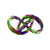
> f:=51344*y^5+53384*y^4-47264*y^3-415912*x^2*y^3-49304*y^2+29070*x^2*y^2+247631
> *x^2*y+90164*x^4*y+73931*x^2+40396*x^4;
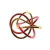
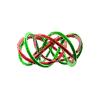
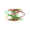
> plot_knot(f,x,y,lightmodel=light4,shading=ZHUE);
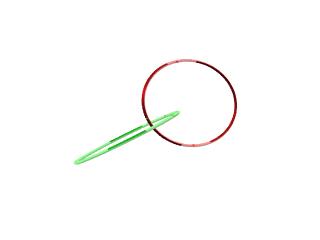
The curve f is irreducible and so it consists of only 1 component. But locally around the point 0 it has 2 components. To see this in the second picture at the top of this page, imagine that you could only see a very small environment around the point x=0, y=0 and nothing else. Then the curve would look like two intersecting lines. So even though the curve is globally irreducible, locally around the point 0 it is reducible and consists of 2 components.
Information on these components and their intersection multiplicities can be given in the form of Puiseux pairs, obtained by computing the Puiseux expansions. A different way to represent this information is as follows: By identifying C^2 with R^4 the curve can be viewed as a 2 dimensional surface over the real numbers. Now we can draw a small sphere inside R^4 around the point 0. The surface of the sphere has dimension 3 over R. The intersection with the curve (which has dimension 1 over the complex numbers, so dimension 2 over the real numbers) consists of a number of closed curves over the real numbers, inside a space (the sphere surface) of dimension 3. After applying a projection from the sphere surface to R^3 these curves can be plotted. See also: E. Brieskorn, H. Knörrer: Ebene Algebraische Kurven , Birkhäuser 1981.
In this plot, each component will correspond to one of the local components. Furthermore the winding number in the plot equals the intersection multiplicity of the two branches of the curve. In this example this number is 1. In case we want to see more complicated 3D plots, we only need to make the singularity more complicated and the intersection multiplicities of the branches higher. Since we are only interested in the curve locally, it does not matter if the curve is irreducible or not. However, the input of plot_knot must be squarefree.
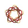
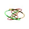
> plot_knot(y^3-x^2,x,y);
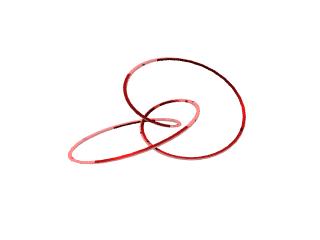
We see that a cusp gives a 2-3 torus-knot. More generally, if igcd(p,g)=1 then plot_knot(x^p-y^q,x,y) gives a p-q torus-knot.
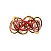
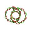
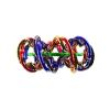
It gets more interesting if we have plots consisting of more components. For this, we only need to have a singularity consisting of more components. In this example we start with a 2-3 torus-knot, using y^3-x^2. To obtain a high intersection multiplicity we add a high power of x and multiply these two components. Then we get:
> plot_knot((y^3-x^2)*(y^3-x^2-x^10),x,y,colours=[blue,yellow],numpoints=500,
> lightmodel=light4,orientation=[0,0]);
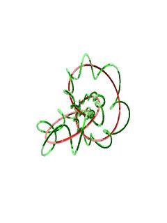
It sometimes requires some tweaking with the various options (see the help page of plot_knot), or to change some of the coefficients (for example the coefficient of x^10) to get good pictures. They tend to look best when viewed from straight angles (the numbers theta and phi in the plot window are 0 or 90) and when using the light schemes under the color menu.
animation:Java |
animation:Java |
animation:Java |
animation:Java |
animation:Java |
animation:Java |
animation:Java |
animation:Java |
animation:Java |
> f:=y^4-(x^4-x^3-2*x^2);
                                  4    4    3      2
                            f := y  - x  + x  + 2 x
> genus(f,x,y);
1
> w:=Weierstrassform(f,x,y,x0,y0);
                                   2                     2
         2     3                  y             y      x0  + 288        y0
 w := [y0  + x0  + 288 x0, -24 ---------, 144 -----, 2 ---------, 12 ---------]
                               x (x - 2)      x - 2      2             2
                                                       x0  - 576     x0  - 576
> j_invariant(f,x,y);
1728
For curves with genus 0 one can compute a parametrization, a
bijection between the curve and a projective line. One can view this
projective line as a normal form for curves with genus 0. For
curves with genus 1 we can also compute a normal form, the Weierstrass
normal form. In this form the curve is written as: y^2 - (polynomial
in x of degree 3). To avoid ambiguity we will denote the
Weierstrass normal form with the variables x0 and y0 instead
of x and y.
> f0:=w[1];
                                    2     3
                            f0 := y0  + x0  + 288 x0
Now the curves f and f0 are birationally equivalent. The
Weierstrassform algorithm computes such an equivalence in two directions,
namely [w[2] , w[3]] is a morphism from f to f0 and
[w[4] , w[5]] is the inverse morphism. Let's check this for the
point (-2,2,1) on f.
> subs(x=-2,y=2,[w[2],w[3]]);
[-12, -72]
Now check if this is on f0:
> subs(x0="[1],y0="[2],f0);
0
OK. Now try the inverse, and see if we get the point (-2,2,1):
> subs(x0=""[1],y0=""[2],[w[4] , w[5]]);
[-2, 2]
OK.
Other Maple packages: CASA and algcurve.
CASA: This package contains code for curves and for other algebraic varieties as well. algcurve: The Maple share library contains a different package on algebraic curves, called algcurve. It can be loaded into Maple by the commands: with(share): readshare(algcurve,geometry): with(algcurve);