EXAMPLE 3.2.1
To paraphrase Benjamin Disraeli: "There are lies, darn lies, and DAM STATISTICS."
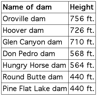
Compute the mean, median and mode for the following DAM STATISTICS:
A measure of central tendency is a number that represents the typical value in a collection of numbers. Three familiar measures of central tendency are the mean, the median, and the mode.
We will let n represent the number of data points in the distribution. Then
![]()
(The mean is also known as the "average" or the "arithmetic average.")
Median = "middle" data point (or average of two middle data points) when the data points are arranged in numerical order.
Mode = the value that occurs most often (if there is such a value).
In EXAMPLE 3.2.1 the distribution has 7 data points, so n = 7.
MEAN = (756 + 726 + 710 + 568 + 564 + 440 + 440)/7
= 4204/7 = 600.57 (this has been rounded).
We can say that the typical dam is 600.57 feet tall.
We can also use the MEDIAN to describe the typical response. In order to find the median we must first list the data points in numerical order:
756, 726, 710, 568, 564, 440, 440
Now we choose the number in the middle of the list.
756, 726, 710, 568, 564, 440, 440
The median is 568.
Because the median is 568 it is reasonable to say that on this list the typical dam is 568 feet tall. Notice that there were just as many dams that are 568 feet tall or taller as there are dams that are 568 feet tall or shorter.
We can also use the MODE to describe the typical dam height. Since the number 440 occurs more often than any of the other numbers on this list, the mode is 440.
EXAMPLE 3.2.2
Survey question: How many semester hours are you taking this semester?
Responses: 15, 12, 18, 12, 15, 15, 12, 18, 15, 16
What was the typical response?
see solution
FINDING THE "MIDDLE" OF A LIST OF NUMBERS
In the two previous examples, we found the median by first arranging the list numerically and then crossing off data points from each end of the list until we arrived at the middle. This method works well as long as there are relatively few data points to work with. In cases where we are dealing with a large collection of data, however, it is not a practical method for finding the median.
If n represents the number of data points in a distribution, then:
the position of the "middle value" is
If the data points have been arranged numerically, we can use this fact to efficiently find the median.
Example:
For the following list, n = 19.
24, 25, 28, 31, 33, 33, 36, 42, 42, 48, 51, 57, 57, 68, 75, 79, 79, 79, 85
The numbers are already in numerical order. The position of the "middle of the list" is:
(n+1)/2 = (19+1)/2 = 20/2 =10
Thus, the tenth number will be the median:
24, 25, 28, 31, 33, 33, 36, 42, 42, 48, 51, 57, 57, 68, 75, 79, 79, 79, 85
The median is 48.
EXAMPLE 3.2.3
Compute the mean, median, and mode for this distribution of test scores:
92, 68, 80, 68, 84
see solution
FREQUENCY TABLES
EXAMPLE 3.2.5
Find the mean, median and mode for the following collection of responses to the question: "How many parking tickets have you received this semester?"
1, 1, 0,1, 2, 2, 0, 0, 0, 3, 3,0, 3, 3, 0,2, 2, 2, 1, 1,4, 1, 1,0,3, 0, 0, 0, 1, 1, 2, 2, 2, 2,1, 1, 1, 1, 4, 4, 4,1, 1, 1, 1, 2, 2, 2, 2, 2, 2, 2, 2,1, 1, 1, 1, 1, 3,3,0, 3, 3, 1, 1, 1, 1,0, 0, 1, 1, 1, 1, 3, 3, 3, 2, 3, 3, 1, 1, 1,2, 2, 2,4, 5, 5, 4, 4, 1, 1, 1, 4,1, 1, 1,3, 3, 5,3, 3, 3, 2,3, 3, 0, 0, 0, 0, 3, 3, 3, 3, 3, 3, 0, 2, 2, 2, 2, 1, 1, 1,3, 1, 0, 0, 0,1, 1, 3,1, 1, 1, 2, 2, 2, 4, 2, 2, 2, 1, 1, 1, 1,0, 0, 2, 2, 3, 3,2, 2, 3,2, 0, 0, 1, 1,3, 3, 3, 1, 1, 1, 1, 1,2, 2, 2, 2, 1, 1, 1, 1, 0,1, 1, 1, 3,1, 1, 1, 2, 2, 2, 1, 1, 1,2, 1, 1, 1,3, 3,5, 3, 3, 1, 1, 1, 3, 3, 3, 3, 1, 1, 1,4, 1, 1, 4, 4, 4, 4, 4, 4,1, 1, 1,2, 2,5, 5, 2, 3, 3, 4, 4,3,2, 2, 2, 1,5, 1,2, 2, 1, 1, 1, 2, 2, 2, 2, 2,1, 1, 0,1, 1, 1,3, 3, 3, 3, 3
EXAMPLE 3.2.5 SOLUTION
It will be much easier to work with this unwieldy collection of data if we organize it first. We will arrange the data numerically.
0, 0, 0, 0, 0, 0, 0, 0, 0, 0, 0, 0, 0, 0, 0, 0, 0, 0, 0, 0, 0, 0, 0, 0, 0, 0, 0,
1, 1, 1, 1, 1, 1, 1, 1, 1, 1, 1, 1, 1, 1, 1, 1, 1, 1, 1, 1, 1, 1, 1, 1, 1, 1, 1, 1, 1, 1, 1, 1, 1, 1, 1, 1, 1, 1, 1,
1, 1, 1, 1, 1, 1, 1, 1, 1, 1, 1, 1, 1, 1, 1, 1, 1, 1, 1, 1, 1, 1, 1, 1, 1, 1, 1, 1, 1, 1, 1, 1, 1, 1, 1, 1, 1, 1, 1,
1, 1, 1, 1, 1, 1, 1, 1, 1, 1, 1, 1, 1, 1, 1, 1, 1, 1,
2, 2, 2, 2, 2, 2, 2, 2, 2, 2, 2, 2, 2, 2, 2, 2, 2, 2, 2, 2, 2, 2, 2, 2, 2, 2, 2, 2, 2, 2, 2, 2, 2, 2, 2, 2, 2, 2, 2, 2, 2, 2, 2, 2, 2, 2, 2, 2, 2, 2, 2, 2, 2, 2, 2, 2, 2, 2,
3, 3, 3, 3, 3, 3, 3, 3, 3, 3, 3, 3, 3, 3, 3, 3, 3, 3, 3, 3, 3, 3, 3, 3, 3, 3, 3, 3, 3, 3, 3, 3, 3, 3, 3, 3, 3, 3, 3, 3, 3, 3, 3, 3, 3, 3, 3, 3, 3, 3, 3, 3, 3, 3,
4, 4, 4, 4, 4, 4, 4, 4, 4, 4, 4, 4, 4, 4, 4, 4, 4, 4,
5, 5, 5, 5, 5, 5, 5
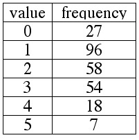
The value "0" appears 27 times.
The value "1" appears 96 times.
The value "2" appears 58 times.
The value "3" appears 54 times.
The value "4" appears 18 times.
The value "5" appears 7 times.
We can summarize the information above in the following frequency table:
A frequency table is a shorthand representation of list of data.
The numbers in the "value" column indicate which numbers appear on the original list of data.
The numbers in the "frequency" column tell how many times the corresponding value appears
on the original list of data.
Now we find the mean, median and mode for the data in the table.
MODE
The mode, if it exists, is easiest to find. For data presented in a frequency table,
the mode is the value associated with the greatest frequency (if there is a greatest frequency).
In this case, the greatest frequency is 96 and the associated value is "1,"
so the mode is "1." More students received 1 parking ticket than any of the
other possibilities.
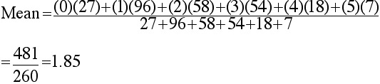
MEAN
To find the mean, we must have a convenient way to determine the sum
of all the data points, and also a convenient way to determine n, the
number of data points in the distribution. We may be tempted to merely
add the six numbers in the "value" column, and divide by six, but that
would be incorrect, because it would fail to take into account that facts
that the distribution includes many more than just six data points,
and the various values do not all occur with the same frequency.
To find n in a case like this, we find the sum of numbers in the "frequency" column.
This makes sense, when we recall that the frequencies tell
how many times each of the values occurs.
n = sum of frequencies = 27 + 96 + 58 + 54 + 18 + 7 = 260
The mean will be the sum of all 260 data points, divided by 260.
Finding the sum of all 260 data points is simpler than it may at first seem, when we
recall what the table represents. For example, since the value 0 has a frequency of 27,
when we took the sum of all of the zeroes in the distribution,
that subtotal would be (0)(27) = 0. Summarizing the process described above, we have the following general rule for
determining the mean for data in a frequency table:
Mean = S/n
where n, the number of data points in the distribution, is obtained by
finding the sum of all of the frequencies, and S, the sum of the data points,
is found by adding all of the subtotals formed by multiplying a value by its
associated frequency.
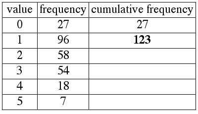
Next we would read all of the 1s from the list. There are 96 of them.
Thus, after we have read all the 0s and 1s from the list,
we would have read a total of 27 + 96 = 123 numbers.
We summarize this by saying that the value 1 has a cumulative frequency of 123.
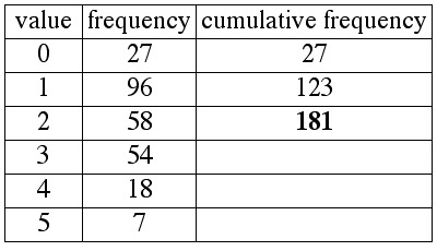
Continuing this process, after having read all of the 0s and 1s from the list,
we would read all of the 2s from the list. Since the value 2 appears on the list 58 times,
after we read all of the 0s, 1s and 2s from the list,
we will have read a total of 27 + 96 + 58 = 181 numbers.
We say that the value 2 has a cumulative frequency of 181.
At this point we will stop. Remember, the reason we started making the column for
cumulative frequency was so that we could locate the 130th and 131st numbers, in order to
determine the median. Now we see that the 130th and 131st numbers are both
2s (the cumulative frequency column tells us, in fact,
that the 124th through 181st numbers on the list are all 2s).
The two middle numbers are both 2s, so the median is 2.
Now this table conveys everything that was significant about the distribution of data
that we presented at the beginning of this example. When working with frequency tables,
recall this fundamental fact:
Likewise, the second row in the table shows use that the value 1 appears 96 times
in the distribution, so when we took the sum of all of the ones, we would get a
subtotal of (1)(96) = 96.
Continuing in this vein, the next row of the table
tells us that the value 2 appears in the distribution 58 times, so when we took
the sum of all of the twos from the list, we would have a subtotal of (2)(58) = 116.
This indicates that in order to find the sum of all of the data points in a frequency
table, we find the sum of all subtotals formed by multiplying a value times its frequency.
MEDIAN
To find the median, we need to recall that we are trying to find the
middle number (or two middle numbers) in a list of 260 numbers.
Recall from earlier that the position of the middle number
is ![]()
In this case, the position of the middle number is ![]()
Since 130.5 is located between 130 and 131, the median will be the average of the 130th and 131st numbers
in the ordered list (by the way, since the values are arranged numerically in the table as
we read from top to bottom, this data has already been ordered). We need to count through
the table until we find the 130th and 131st numbers. This is done as follows, by taking
into account the cumulative frequency as the values in the various rows are "read" from the table.
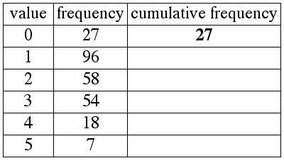
To make a column for cumulative frequency, we pretend that we are reading data from a list,
in numerical order. If we were to do so, the first 27 numbers on the list would all be "0."
This means that after all of the 0s are read from the list, we would have read a total of 27 numbers.
We say that the value 0 has a cumulative frequency of 27:
From the previous example we generalize to form this rule for determining
the median for data in a frequency table (this rule assumes that the values
appear in the table in numerical order).
Make a column for cumulative frequency as follows:
1. The cumulative frequency of the first row is the same as the frequency of the first row.
2. For every other row, determine cumulative frequency by adding the frequency of that
row to the cumulative frequency of the previous row.
When cumulative frequency first equals or exceeds ![]()
![]() is exactly .5 greater than one of the cumulative frequencies, then the median will be the average of the associated values from that row and the next row).
is exactly .5 greater than one of the cumulative frequencies, then the median will be the average of the associated values from that row and the next row).
EXAMPLE 3.2.6
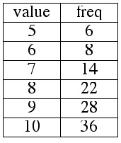
The frequency table below represents the distribution of scores on a ten-point quiz.
Compute the mean, median, and mode for this distribution.
Quiz Scores
see solution
EXAMPLE 3.2.7
The frequency table below represents the distribution, according to age, of students in a certain class.
Ages of Students
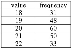
1. Find the mean, median, and mode for this distribution.
2. True or false: 18 students were 31 years old.
EXAMPLE 3.2.8
Members of the preview audience for the new Arnie Schvartzengagger film,
The Predagagger XII: Things Blow Up, were asked to rank the film from 0 ("stinks like a dead cyborg") to 6 ("XII thumbs up!"). The results are summarized in the table below.
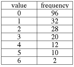
1. True or false: The median is 3.
2. True or false: The mean is 3.
3. True or false: Twenty-eight people gave the film a rank of 2.
4. True or false: 128 people gave the film a rank of less than 2.
see solution
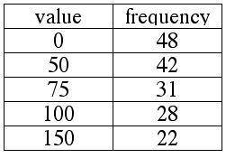
EXAMPLE 3.2.9
A number of people invested $1000 each in the Gomer Family of Mutual Funds.
The frequency table below shows the current values of those investments.
Compute the mean, median and mode.
see solution
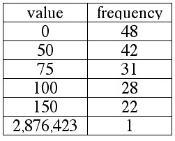
EXAMPLE 3.2.10
A number of people invested $1000 each in the Gomer Family of Mutual Funds.
The frequency table below shows the current values of those investments after
Gomer hit the trifecta at the dog track, and hit the Cash 5 jackpot.
Compute the mean, median and mode.
see solution
EXTREME VALUES and THEIR EFFECTS ON MEAN, MEDIAN and MODE
If we compare the previous two examples, we see that the two distributions are nearly identical,
except that the distribution in EXAMPLE 3.2.10 contains one extra number (2,876,423) that is
significantly greater than any of the other numbers in the distribution.
(A number that is significantly greater or significantly less than most of the other numbers in a
distribution is called an extreme value or outlier.)
Notice that including this extreme value had a huge effect on the mean of the distribution
(which increased from $61.55 to $16,784.58) but had no effect whatsoever on
either the median or the mode. Also notice that in the distribution in EXAMPLE 2.1.10,
the mean is not a good representation of the typical value in the distribution.
This illustrates an important general fact:
Of the three measures of central tendency (mean, median, mode), the mean is the
measure that is most likely to be distorted by the presence of extreme values.
EXAMPLE 3.2.11
The annual earnings for employees of a certain restaurant are given below:
12 laborers earn $8000 each.
10 laborers earn $9000 each.
4 supervisors earn $11000 each
The owner/manager earns $240,000.
Of the three measures of central tendency, which will be the least accurate representation of
"typical earnings?"
see solution
Download practice exercises (PDF file)