Lecture 13: Projective Structures on Surfaces Part III

Last time we discussed how one could convexly glue convex projective structures on surfaces along principal boundary components. We also discussed the moduli space of such gluings. In this lecture we will show how to explicitly parametrize convex projective structrues with principal boundary on a pair of pants. This will complete the proof of the following theorem:

Theorem 1: Let \(\Sigma\) be a closed surface of genus \(g\geq 2\). The space \(\mathfrak{B}(\Sigma)\) of marked convex projective structures on \(\Sigma\) is a cell of dimension \(16g-16=8\vert \chi(\Sigma)\vert\)

The proof of this theorem involves a double induction on the Euler characteristic and number of boundary components. The base case of which the case of a pair of pants \(P\). Specifically, we prove the following.

Theorem 2: The space \(\mathfrak{B}(P)\) of marked convex projective structrures on \(P\) with principal boundary components is a cell of dimension 8.

The proof of Theorem 2 consists of constructing an explicit system of coordinates. In order to define these coordinates, we first need a diversion into flags in vector spaces.

####Flags

Let \(V\) be a real vector space of dimension \(n\). A complete flag in V, \(\{F_i\}_{i=0}^n\), is a collection of subspace of \(V\) such that

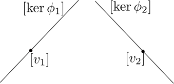
such that \(\dim(F_i)=i\). Since flags are defined using subspaces we can think of a flag as a collection of projective subspaces and thus as a subset of \(P(V)\). We will primarily be concerned with flags in \(\mathbb{R}P^2\), and such flags admit a convenient alternate description. It easy to see that flags in \(\mathbb{R}P^2\) can be thought of as the set

Before we proceed, we need to describe a collection of flags being in “general position.” Let \((\{F^1_i\},\ldots \{F^k_i\})\) be a \(k\)-tuple of flags in \(\mathbb{R}P^2\) and let \(\{i_j\}_{j=1}^k\) a collection of \(k\) non-negative integers that sum to \(3\). Then this \(k\)-tuple is generic if \(\dim(F^1_{i_1}+\ldots+F^k_{i_k})=3\). Or is other words, the subspaces of the flags span subspaces that are as large as their dimensions allow. Below is a generic pair of flags in \(\mathbb{R}P^2\).

There is an obvious \(SL_3(\mathbb{R})\) action on the space of \(k\)-tuples of flags in \(\mathbb{R}P^2\). We define the configuration space of \(k\)-tuples of flags, which we denote \(Conf_k\), as the quotient of the space of \(k\)-tuples of flags by the \(SL_3(\mathbb{R})\) action. More important for our purposes will be the space \(Conf^\ast_k\subset Conf_k\) consisting of configurations of generic \(k\)-tuples of flags.

We now describe the configuration spaces of \(k\)-tuples of generic flags for small values of \(k\). Let \(\{F_i\}\) be a flag in \(\mathbb{R}P^2\) and let \(S=\{v_1,v_2,v_3\}\) be a basis of \(\mathbb{R}^3\). Then \(S\) is adapted to \(\{F_i\}\) if \(Span(\{v_1,\ldots, v_k\})=F_k\) for \(1\leq k\leq 3\). Using adapted bases, it is easy to see that \(SL_3(\mathbb{R})\) acts transitively on the space of flags in \(\mathbb{R}P^2\). As a result we see that \(Conf_1^\ast\) is a point. The stabilizer of a flag \(\{F_i\}\) under this action is the subgroup \(B\) of upper triangular matrices with respect to an adapted basis for \(\{F\}\).

Let

It can be easily verified that \(B\) acts transitively on \(R_{\{F_i\}}\), and as a result we see that \(Conf^\ast_2\) is also a point. Furthermore, if we consider the generic pair \((([e_1],[e_3^\ast]),([e_3],[e_1^\ast]))\) then we see that the stabilizer of this pair in \(SL_3(\mathbb{R})\) consists of diagonal matrices with respect to the standard basis. As a results we see if we are given a generic triple of flags \(((p_1,\phi_1),(p_2,\phi_2),(p_3,\phi_3))\), then we can assume that \(p_1=[e_1]\), \(p_2=[e_3]\), \(\phi_1=[e_3^\ast]\), and \(\phi_2=[e_3^\ast]\). Furthermore, by genericity we know that \(p_3\) is not contained in any of the lines spanned by any pair of the standard basis vectors. Since \(D\) acts simply transitively on the complement of these lines we can move \(p_3\) to \([e_1+e_2+e_3]\) and assume that for some \(d\in \mathbb{R}\) that \(\phi_3=[de_1^\ast+(-1-d)e_2^\ast+e_3^\ast]\). At this point we have normalized our flags as much as possible and so we see that \(Conf_3^\ast\) is one dimensional and is parameterized by \(d\). However, not all values of \(d\) are admissible. When \(d=0\) \(\phi_3\) contains \([e_1]\) and is thus not generic and when \(d=-1\) \(\phi_3\) contains \([e_2]\) and is thus not generic. All other values of \(d\) give generic triples and so we see that

Lemma: \(Conf_3^\ast\cong \mathbb{R}\setminus \{0,-1\}\).

There is an equivalent, but more invariant way of parameterizing \(Conf_3^\ast\). Let \(((p_1,\phi_1),(p_2,\phi_2),(p_3,\phi_3))\) be a triple of generic flags. By abuse of notation we will think if the \(p_i\) as elements of \(\mathbb{R}^3\) and the \(\phi_i\) as elements of \(\mathbb{R}^{3\ast}\). Then we define the triple ratio of the triple of flags as

A simple computation shows that if we normalize our flags as above then their triple ratio is equal to \(d\). It is also easy to check that the triple ratio is an \(SL_3(\mathbb{R})\)-invariant function on triples of flags. Henceforth, we will think of generic triples as being parameterized by their cross ratio.

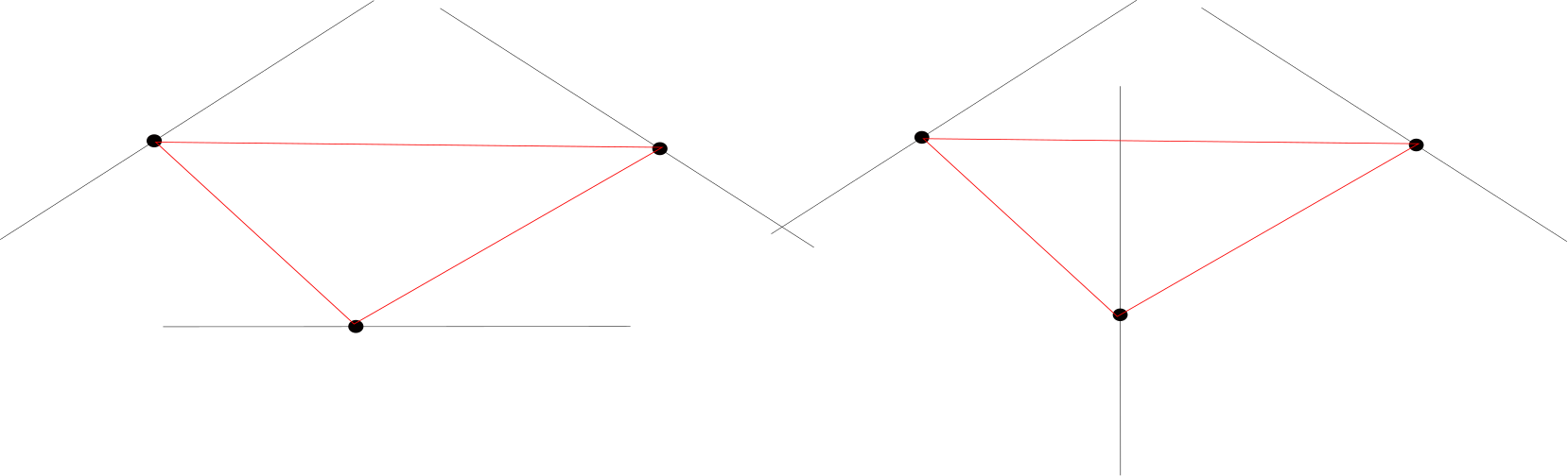
We now take a moment to discuss the qualitiative difference between triples with positive and negative triple ratios. When the triple has positive triple ratio it is possible to find a triangle component of the complement of the region spanned by the point parts of the three flags that is disjoint from the lines coming from the three flags. When the triple ratio is negative the line components of the flags intersect all four possible triangles. Below we see an example of a triple with positive triple ratio (left) and with negative triple ratio (right).

Finally, we discuss how to parameterize \(Conf_4^\ast\). We will prove the following lemma

Lemma: \(Conf_4^\ast\cong (\mathbb{R}\setminus\{0,-1\})^4\).

Let \(((p_i,\phi_i))_{i=1}^4\) be an element of \(Conf_4^\ast\) and assume without loss of generality that \(p_1=[e_1]\), \(p_2=[e_3]\), \(p_3=[e_1+e_2+e_3]\), \(\phi_1=[e_3^\ast]\), and \(\phi_2=[e_1^\ast]\). With reference to the figure below we let \(c_1\) and \(c_4\) be the triple ratios of the flags \(((p_i,\phi_1))_{i=1}^3\) and \(((p_i,\phi_i))_{i=2}^4\), respectively. We also, let \(c_2\) be the cross ratio of the 4 concurrent lines \(\phi_1\), \([p_1,p_3]\), \([p_1,p_2]\), \(\ell_1\), normalized in a projective coordinate system where the first three lines correspond to \(\infty\), \(-1\), and \(0\). Finally, we let \(c_3\) be the cross ratio of the 4 concurrent lines \(\phi_2\), \([p_2,p_3]\), \([p_2,p_1]\), \(\ell_2\), again normalized so that the first three lines correspond to \(\infty\), \(-1\), and \(0\). As a result we see that an element of \(Conf_4^\ast\) determines 4 real numbers described above. It is a simple calculation to show that genericity of these flags implies that none of these numbers is either \(-1\) or \(0\).

We now show that given four number \(c_1\), \(c_2\), \(c_3\), and \(c_4\) that we can determine a unique flag giving rise to these invariants. Again we reference the figure below. Since the triple ratio determines a triple of flags we can use \(c_1\) to determine \(\phi_3\). If we knew the position of \(p_4\) we could use the triple ratio \(c_4\) to determine \(\phi_4\) and then the flag would be completely determined. We now show how we can use \(c_2\) and \(c_3\) to determine \(p_4\). It is easy to see that \(p_4=\ell_1\cap\ell_2\). However, once we know \(c_2\) we can recover \(\ell_1\) and once we know \(c_3\) we can recover \(\ell_2\).

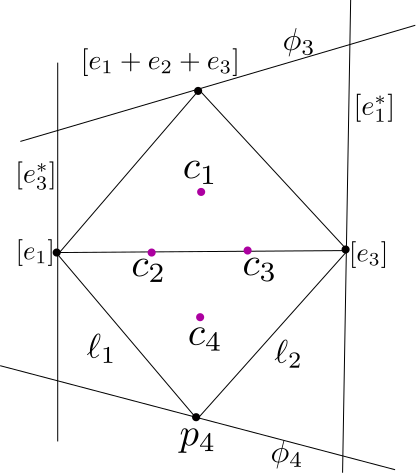
We now discuss some qualitative differences that occur when the values of the \(c_i\) are positive. When all of the numbers are positive, the point components of the flags form the boundary of a quadrilateral that is disjoint from the flag components of all of the flags. This is illustrated in the above figure. The picture is less nice when some of the corrdinates are negative. For example, if \(c_2\) and \(c_3\) are negative the point \(p_4\) is contained in one of the triangles spanned by \(p_1\), \(p_2\), and \(p_3\).

We now show how we can use these coordinates to parameterize convex projective structures with principal boundary on pairs of pants. Let \(Q=(\mathbb{R}^+)^8\).

Theorem: \(\mathfrak{B}(P)\cong Q\).

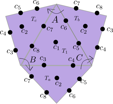
Proof sketch: Given a pair of pants \(P\), it is possible to decompose \(P\) into ideal triangles \(\tau_1\) and \(\tau_2\) by cutting along 3 curves spiraling along the various boundary components. We can label the faces of these two triangles with numbers \(c_1\) and \(c_2\) and use 6 additional numbers to label the three edges of the triangulation (with two numbers each). We can lift this triangulation as well as the labelling to the universal cover \(\tilde P\). Using the labelings on the triangulation of \(\tilde P\) we can define the developing map for a projective structure by building the flags in \(\mathbb{R}P^2\) dictated by the numbers decorating the triangulation. By construction we see that since the coordinates are positive we can realize the image of our developing map as an increasing union of convex sets and thus the entire image is convex. The fundamental group is generated by curves \(A\), \(B\), and \(C\) encircling the boundary components of \(P\) and so \(\pi_1P=\langle A,B,C\mid ABC=1\rangle\). If \(T_1\) is a lift of \(\tau_1\) then there are three adjacent copies of \(\tau_2\) to \(\tilde P\) which we denote \(T_a\), \(T_b\), and \(T_c\). The convention being that \(A\) takes \(T_b\) to \(T_c\) and a similar convention for the other triangles. This configuration is shown below. Since there is a unique projective transformation between any pair of triples of generic flags with the same triple ratio, we see that we can also define the holonomy representation for this projective structure.

Conversely, given a convex projective structure on \(P\) with principal boundary components, we can produce an equivariant collection of flags (where the flag at each vertex is dictated by the holonomy fixing that vertex). Since the developing map of this structure is injective with convex image we see that the cooridinates for our flags must all be positive.

Previous Post: Lecture 12: Projective Structures on Surfaces Part II

Next Post: Lecture 14: Deforming Strictly Convex Projective Manifolds